In the last article, we provides a full set-theoretic interpretation for typed lambda calculus based on the Henkin model. However, the function recursion in PCF is hard to model from a pure set view. To solve this problem, we need to introduce a new class of models that are based on partially-ordered structures, called domains. And such models are called domain-theoretic models.
Before diving into the new model, in this article, we focus on introducing two necessary concepts: one is the complete partial order (CPO), which is the simplest class of domains; another one is the continuous function, which is very useful when we discuss properties of recursion functions.
To motivate the central properties of domains, we start from an intuitive discussion of recursive definitions.
Recursive Definitions and Fixed Point Operators
Recall from Easy Foundations for Programming Languages III — The Language PCF & Its Syntax that if we wish to add a recursive definition form
\[\text{letrec } f:\sigma = M \text{ in } N\]to typed lambda calculus, it suffices to add a fixed-point operator $fix_\sigma$ that returns a fixed point of any function from $\sigma$ to $\sigma$.
Therefore, we study a class of models for $\lambda^{\times,\to}$, and extensions, in which functions of the appropriate type have fixed points. A specific example will be a model (denotational semantics) of PCF.
We will use properties of ($fix$) reduction to motivate the semantic interpretation of $fix$. To emphasize a few points about ($fix$) reduction, we will review the factorial example discussed in that article. In this example, we assume reduction rules for conditional, equality test, substraction and multiplication.
Using $fix_{nat \to nat}$, the factorial function may be written \(fact \:\stackrel{\text{def}}{=} \: fix_{nat \to nat} \: F\), where $F$ is the expression
\[F \:\stackrel{\text{def}}{=} \: \lambda f:nat \to nat.\: \lambda y:nat.\: \text{if } Eq? \: y \: 0 \text{ then } 1 \text{ else } y*f(y-1).\]Since the type is clear from context, we will drop the subscript from $fix$. To compute \(fact \: n\), we expand the definition, and use reduction to obtain the following.
\[\begin{split} fact \: n &= (\lambda f : nat \to nat .\: f(fix \: f)) \: F \: n\\ &= F \: (fix \: F) \: n \\ &= (\lambda f:nat \to nat.\: \lambda y:nat.\: \text{if } Eq? \: y \: 0 \text{ then } 1 \text{ else } y*f(y-1))\: (fix \: F) \: n \\ &= \text{if } Eq? \: n \: 0 \text{ then } 1 \text{ else } n*(fix \: F)(n-1) \end{split}\]When $n=0$, we can use the reduction axiom for conditional to simplify $fact$ $0$ to $1$. For $n > 0$, we can simplify the test to obtain \(n*(fix \: F)(n-1)\), and continue as above. For any numeral $n$, we will eventually reduce $fact$ $n$ to the numeral for $n!$.
An alternative approach to understanding $fact$ is to consider the finite expansions of $fix$ $F$.
To make this as intuitive as possible, let us temporarily think of $nat \to nat$ as a collection of partial functions on the natural numbers, represented by sets of ordered pairs. Using a constant $diverge$ for the “nowhere defined” function (the empty set of ordered pairs). we let the “zero-th expansion” \(fix^{[0]} \: F = diverge\) and define
\[fix^{[n+1]} \: F = F \:(fix^{[n]} \: F )\]In computational terms, $fix^{[n]}$ $F$ describes the recursive function computed using at most $n$ evaluations of the body of $F$. Or, put another way, $fix^{[n]}$ $F$ is the best we could do with a machine having such limited memory that allocating space for more than $n$ function calls would overflow the run-time stack.
For example, we can see that \((fix^{[2]} \: F)\:0=1\) and \((fix^{[2]} \: F)\:1=1\), but \((fix^{[2]} \: F)\:n\) is undefined for $n \geq 2$. This reflects the fact that if we are allowed more recursive calls, we may compute factorial for larger natural numbers.
An intuitive way to specify the meaning of $fix$ is to let \(fact =\bigcup_n fix^{[n]} \: F\); this gives us the standard factorial function. However, there is no reason to believe that for arbitrary $F$, \(\bigcup_n fix^{[n]} \: F\) is a fixed point of $F$. This may be guaranteed by imposing some conditions on $F$.
A specific problem related to recursion is the interpretation of terms that define nonterminating computations. Since recursion allows us to write expressions that have no normal form, we must give meaning to expressions that do not seem to define any standard value. For example, it is impossible to simplify the PCF expression
\[\text{letrec } f:nat \to nat = \lambda x:nat .\: f(x+1) \text{ in } f \: 3\]to a numeral, even though the type of this expression is $nat$. It is sensible to give this term type $nat$, since it is clear from the typing rules that if any term of this form were to have a normal form, the result would be a natural number. Rather than say that the value of this expression is undefined, which would make the meaning function on models a partial function, we extend the domain of “natural numbers” to include an additional value $\perp_{nat}$ to represent nonterminating computations of type $nat$. This gives us a way to represent partial functions as total ones, since we may view any partial numeric function as a function into the domain of natural numbers with $\perp_{nat}$ added.
Partial Orders
To enable the expansion of $F$ in the \(fix^{[i]} \: F\) style and introduce the additional value $\perp_{nat}$ as we discussed in the last section, we need the help of partial ordering.
Basic Definitions
A partial order $\langle D, \leq \rangle$ is a set $D$ with reflexive, anti-symmetric and transitive relation $\leq$.
Reflexivity means that $d \leq d$ for every $d \in D$, and transitivity means that if $d \leq d’$ and $d’ \leq d’’$, then $d \leq d’’$. A relation is anti-symmetric if $d \leq d’$ and $d’ \leq d$ imply $d=d$. Antisymmetry implies that there are no “loops” $d \leq d’ \leq d$ with $d \neq d’$.
Any set can be considered a partial order using the discrete order $x \leq y$ iff $ x = y $. Intuitively, discrete order means that no relation exists between distinct elements.
If any any two elements are comparable in a partial order, then we call this order total order or linear order.
An example of partial order is the prefix order on sequences. More precisely, let $S$ be any set and let $S^\ast$ be the set of finite sequences of elements of $S$. We say $s \leq_{\text{prefix}} s’$ iff sequence $s$ is an initial segment of sequence $s’$. This gives a partial order $\langle S^\ast, \leq_{\text{prefix}} \rangle$.
If $\langle D, \leq \rangle$ is a partial order, then an upper bound of a subset $S \subseteq D$ is an element $x \in D$ with $y \leq x$ for every $y \in S$. A least upper bound of $S$ is an upper bound which is $\leq$ every upper bound of $S$. It is easy to see that if a subset $S$ of a partial order $D$ has a least upper bound, the least upper bound is unique (by antisymmetry).
Example: Suppose there is a partial order $\langle D, \leq \rangle$ defined as \(D = \{ 1,2,3,4,5,6 \}\) and $\leq$ representing the smaller than relation between natural numbers. Then the upper bound set of the subset \(S = \{1,2,4\}\) is \(\{5,6\}\), and $5$ is the least upper bound.
If $\langle D, \leq \rangle$ is a partial order, then a subset $S \subseteq D$ is directed if every finite $S_0 \subseteq S$ has an upper bound in $S$. One property of directed sets is that every directed set is nonempty. The reason is that even the empty subset of a directed $S$ must have an upper bound in $S$.
It is easy to see that if $S \subseteq D$ is linearly ordered, which means that $x \leq y$ or $y \leq x$ for all $x,y \in S$, then $S$ is directed.
Another example of a directed set is the partial order \(\{ a_0, b_0, a_1, b_1, a_2, b_2, ... \}\) with $a_i \leq a_j, b_j$ and $b_i \leq a_j, b_j$ for all $i < j$. This partial order consists of two linear orders, $a_0 \leq a_1 \leq a_2 …$ and $b_0 \leq b_1 \leq b_2 …$ connected together so that $a_i$ and $b_i$ have upper bounds $a_{i+1}$ and $b_{i+1}$, but no least upper bound.
Complete Partial Orders
A complete partial order, or CPO for short, is a partial order $\langle D, \leq \rangle$ such that every directed set $S \subseteq D$ has a least upper bound, written $\bigvee S$.
It is easy to show that any finite partial order is a CPO! So, any set can be considered a CPO using the discrete order.
A non-example is that with respect to the ordinary arithmetic ordering, the natural numbers are not a CPO. The reason is that the set $\mathbb{N}$ itself is directed, but has no least upper bound. If we add an extra element $\infty$ greater than all the ordinary numbers, then we can have a CPO.
A trivial but very useful fact is that if $S,T \subseteq D$ are directed, and every element of $S$ is $\leq$ some element of $T$, then $\bigvee S \leq \bigvee T$. In particular, $\bigvee S = \bigvee T$ if every element of either set is $\leq$ than some element of the other.
We define the least element of a partial order as the element that is $\leq$ than all the elements. In interpreting $fix$, we will be particularly interested in CPOs that have least elements. The reason is that every continuous function on a CPO with a least element has a fixed point, as we shall see in the next article. (The definition of continuous functions will be given in the next section.)
If $\mathcal{D} = \langle D, \leq \rangle$ is a partial order with least element, then we say $\mathcal{D}$ is pointed. In this case, we write $\perp_D$ for the least element of $D$. When the CPO is clear from context, we will omit the subscript from $\perp_D$.
A simple class of pointed CPOs are the so-called lifted sets. If $A$ is any set, then we write $A_\perp$ for the CPO whose elements are \(A \cup \{ \perp \}\), ordered so that $x \leq y$ iff $x=y$ or $x=\perp$. The CPO $A_\perp$ is commonly called “A lifted.” We may also lift any CPO $\mathcal{D} = \langle D, \leq_D \rangle$. The result, $\mathcal{D}_{\perp}$, has elements \(D \cup \{ \perp \}\), where $\perp$ is distinct from all elements of $D$. We order \(\mathcal{D}_{\perp}\) so that $x \leq y$ iff $x=y$ or $x,y \in D$ with $x \leq_D y$.
It is easy to see that if $\mathcal{D}$ is a CPO then \(\mathcal{D}_{\perp}\) is a pointed CPO, where the least element is $\perp$.
Two examples that are of particular interest in connection with PCF are \(\mathbb{N}_\perp\) (lifted natural bumbers) and \(\mathbb{B}_\perp\) (lifted booleans). The CPO \(\mathbb{N}_\perp\) looks like this
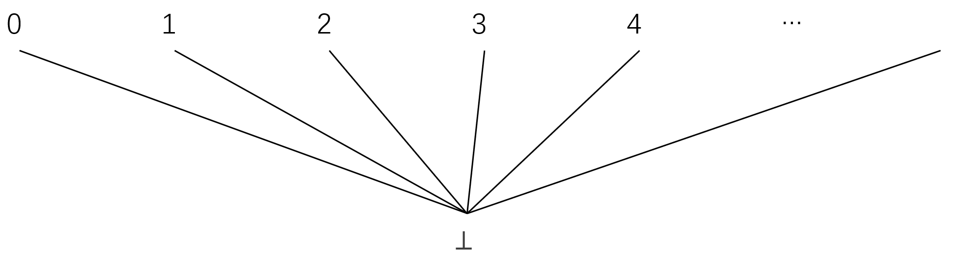
Since this picture is quite flat, a lifted set is sometimes referred to as a flat CPO.
Note: As we mentioned, $\mathbb{N}$ is not a CPO under the arithmetic ordering; however, the lifted version \(\mathbb{N}_{\perp}\) is a CPO. The reason is that, in \(\mathbb{N}_{\perp}\), relations are only defined between a natural numeber and $\perp$, not between two distinct natural numbers.
If $\mathcal{D} = \langle D, \leq \rangle$ and $\mathcal{E} = \langle E, \leq \rangle$ are CPOs, then we may define a cartesian product CPO as follows. We let $\mathcal{D} \times \mathcal{E} = \langle D \times E, \leq_{D \times E} \rangle$, where $D \times E$ is the set of ordered pairs, and the ordering $\leq_{D \times E}$ is defined as follows.
\[\langle d, e \rangle \leq_{D \times E} \langle d', e' \rangle \quad \text{iff} \quad d \leq_D d' \text{ and } e \leq_E e'\]If $S \subseteq D \times E$, it is useful to define sets \(\mathbf{Proj}_1 S = \{ d \mid \langle d, e \rangle \in S \}\) and \(\mathbf{Proj}_2 S = \{ e \mid \langle d, e \rangle \in S \}\).
(Lemma 1.) Suppose $\mathcal{D}$ and $\mathcal{E}$ are CPOs. Their product, $\mathcal{D} \times \mathcal{E}$, is a pointed CPO if both $\mathcal{D}$ and $\mathcal{E}$ are pointed. Moreover, if $S \subseteq D \times E$ is directed, then $\bigvee S = \langle \bigvee \mathbf{Proj}_1 S , \bigvee \mathbf{Proj}_2 S \rangle$.
Before reading the proof, you might find it useful to draw the partial order \(\mathbb{B}_\perp \times \mathbb{B}_\perp\), which has nine elements. Find the least element and check that every directed set has a least upper bound.
(Proof.) We first check that each directed set in $\mathcal{D} \times \mathcal{E}$ has a least upper bound.
Let $S \subseteq D \times E $ be any directed set and define sets $S_1$ and $S_2$ by $S_i = \textbf{Proj}_i S$. We prove the lemma by showing that if $S$ is directed, then $S_1 \subseteq D$ is directed and $S_2 \subseteq D$ is directed. It is then easy to check that the least upper bound of $S$ is the pair \(\langle \bigvee S_1, \bigvee S_2 \rangle\).
To show that $S_1$ is directed, consider any finite subset $T \subseteq S_1$. We must show that $T$ has an upper bound in $S_1$. For every $d \in T$ there is an element $e \in E$ with $\langle d ,e \rangle \in S$, by definition of $S_1$. This means that there is a finite subset $R \subseteq S$ with $\textbf{Proj}_1 R = T$. But since the first component of an upper bound of $R$ gives us an upper bound of $T$, it follows that $T$ has an upper bound in $S_1$. Similar reasoning shows that $S_2$ is also directed.
It is easy to see that if $\mathcal{D}$ and $\mathcal{E}$ have least elements $\perp_D$ and $\perp_E$, then \(\langle \perp_D ,\perp_E \rangle\) is the least element of $\mathcal{D} \times \mathcal{E}$.
$\blacksquare$
Continuous Functions
The continuous functions on CPOs include all of the usual functions we use in programming, and give us a class of functions with fixed points. In this section, we will show that the collection of all continuous functions from one CPO to another forms a CPO. This is an essential step towards constructing a model with each type a CPO. Because in order to do so, function types must be interpreted as CPOs.
Basic Definitions
Suppose $\mathcal{D} = \langle D, \leq_D \rangle$ and $\mathcal{E} = \langle E, \leq_E \rangle$ are CPOs, and $f:D \to E$ is a function on the underlying sets. If $S \subseteq D$. we will write $f(S)$ for the subset of $E$ given by
\[f(S) = \{ f(d) \mid d \in S \}.\]We say $f$ is monotonic if $d \leq d’$ implies $f(d) \leq f(d’)$. It is easy to see that if $f$ is monotonic, and $S$ is directed, then $f(S)$ is directed. A monotonic function $f$ is continuous if, for every directed $S \subseteq D$, we have $f(\bigvee S) = \bigvee f(S)$.
A degenerate but important example is that if $\mathcal{D}$ is discretely ordered, then every function on $\mathcal{D}$ is continuous. A constant function on any CPO is also trivially continuous.
(Lemma 2.) Any monotonic function from a lifted set $A_{\perp}$ to any CPOs is continuous.
(Proof.) In $A_{\perp}$, all nontrivial directed sets have the form \(\{ \perp, a \}\) (because no relation exists between distinct elements of the set $A$) and every monotonic function $f$ must map
\[\begin{split} &\bigvee \{ \perp, a \} = a \text{ to} \\ &\bigvee f(\{ \perp, a \}) = \bigvee \{ f(\perp), f(a) \} = f(a). \end{split}\]$\blacksquare$
It is useful to work out a general construction for continuous functions from one lifted CPO to another. If $\mathcal{D}$ and $\mathcal{E}$ are CPOs, and $f:D \to E$ is continuous, we define the lifted function \(f_\perp : (D \cup \{ \perp \}) \to (E \cup \{ \perp \})\) by
\[f_\perp(d) = \begin{cases} f(d) & \text{if } d \in D \\ \perp & \text{otherwise} \end{cases}\]We summarize the main properties of lifting in the following lemma. If $f$ is a function on pointed CPOs with $f(\perp) = \perp$, then we say $f$ is strict.
(Lemma 3.) Let $\mathcal{D}$ and $\mathcal{E}$ be CPOs. If $f: \mathcal{D} \to \mathcal{E}$ is continuous, then \(f_\perp: \mathcal{D}_\perp \to \mathcal{E}_\perp\) is strict and continuous.
An important special case is that if $A$ and $B$ are sets and $f: A \to B$, then \(f_\perp: A_\perp \to B_\perp\) is a strict continuous function.
(Proof.) A lifted function \(f_\perp: \mathcal{D}_\perp \to \mathcal{E}_\perp\) is strict by definition.
We assume that $f: \mathcal{D} \to \mathcal{E}$ is continuous and show that $f_\perp$ is continuous. To show this, let $S$ be any directed set in \(\mathcal{D}_\perp\). We must show that \(f_\perp(\bigvee S) = \bigvee f_\perp(S)\). The main idea is that either \(S = \{ \perp \}\) or the difference between $f$ and $f_\perp$ does not matter.
If \(S = \{ \perp \}\), then \(f_\perp(\bigvee S) = f_\perp(\perp) = \perp = \bigvee f_\perp(S)\). If \(S \neq \{ \perp \}\), then let $S’ \subseteq D$ be \(S = \{ \perp \}\). Since $S \subseteq D$ and every element of $S’$ is greater than $\perp$ of \(\mathcal{D}_\perp\), we have $\bigvee S = \bigvee S’ \in D$ and $\bigvee f_\perp(S) = \bigvee f_\perp(S’) = \bigvee f(S’)$. Since $f$ is continuous, we have \(f_\perp(\bigvee S) = f(\bigvee S') = \bigvee f(S') = \bigvee f_\perp(S)\). $\blacksquare$
It is worth noting that strict functions are not sufficient to model lambda calculus, and therefore PCF; instead, we need non-strict functions. The reason is that we can define constant functions using lambda calculus, and constant functions do not necessarily map $\perp$ to $\perp$.
In particular, if we interpret $nat$ as the flat CPO $\mathbb{N}_\perp$, the interpretation of \((fix \: \lambda x:nat.\:x)\) will be $\perp$ because it will not terminate. Therefore, the value of the term \((\lambda x:nat.\:3) \: (fix \: \lambda x:nat.\:x)\) will be the result of applying a constant function to $\perp$. However, to be faithful to PCF, the interpretation of this application must be 3, since we can prove \((\lambda x:nat.\:3) \: (fix \: \lambda x:nat.\:x) = 3\), not $\perp$. As a result, we cannot model PCF, or typed lambda calculus, using only strict functions.
Functions as CPO
To asscociate a CPO with each type, we must be able to view the collection of continuous functions from one CPO to another as a CPO. We will partially order functions point-wise, as follows.
Suppose $\mathcal{D} = \langle D, \leq_D \rangle$ and $\mathcal{E} = \langle E, \leq_E \rangle$ are CPOs. For continuous $f,g:D \to E$, we say $f \leq_{D \to E} g$ if, for every $d \in D$, we have $f(d) \leq_E g(d)$. We will write $\mathcal{D} \to \mathcal{E} = \langle D \to E, \leq_{D \to E} \rangle$ for the collection of continuous functions from $\mathcal{D}$ to $\mathcal{E}$, ordered point-wise.
We often say “$f$ is less defined or equal to $g$” when $f \leq_{D \to E} g$.
For example, the semantics of the expression $x+x/x$ is less defined than that of $x+1$, since the former, but not the latter, maps $0$ to $\perp$, and they agree otherwise.
A useful notation is that if $S \subseteq D \to E$ is a set of functions, and $d \in D$, then $S(d) \subseteq E$ is the set given by
\[S(d) = \{ f(d) \mid f \in S \}.\]The above description may seem hard to comprehend, so let us use an example to illustrate the idea.
(Example 1.) There are eleven monotonic functions from $\mathbb{B}_\perp$ to itself, listed in the following table.
| $f(\perp)$ | $f(true)$ | $f(false)$ | |
|---|---|---|---|
| $f_0$ | $\perp$ | $\perp$ | $\perp$ |
| $f_1$ | $\perp$ | $true$ | $\perp$ |
| $f_2$ | $\perp$ | $false$ | $\perp$ |
| $f_3$ | $\perp$ | $\perp$ | $true$ |
| $f_4$ | $\perp$ | $\perp$ | $false$ |
| $f_5$ | $\perp$ | $true$ | $true$ |
| $f_6$ | $\perp$ | $false$ | $true$ |
| $f_7$ | $\perp$ | $true$ | $false$ |
| $f_8$ | $\perp$ | $false$ | $false$ |
| $f_9$ | $true$ | $true$ | $true$ |
| $f_{10}$ | $false$ | $false$ | $false$ |
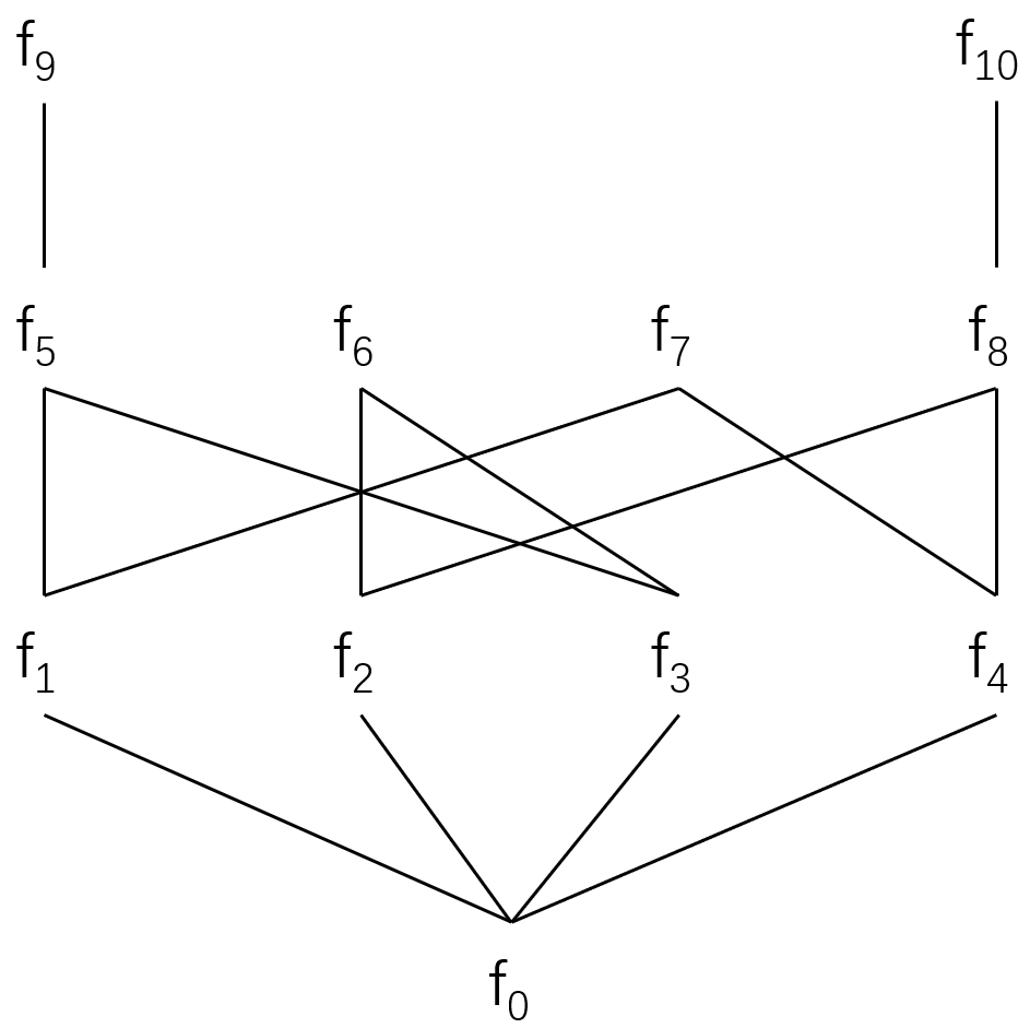
All these functions are continuous due to Lemma 2. In this table, $f_6$ represents the extension of negation: \(not_\perp:\mathbb{B}_\perp \to \mathbb{B}_\perp\). Although $not:\mathbb{B} \to \mathbb{B}$ has no fix point, it is easy to see from the table that $\perp$ is a fixed point of $not_\perp$.
These functions are ordered as shown in the picture below. They constitute a CPO \(\langle \mathbb{B}_\perp \to \mathbb{B}_\perp, \leq_{\mathbb{B}_\perp \to \mathbb{B}_\perp} \rangle\).
(Lemma 4.) For any CPOs $\mathcal{D}$ and $\mathcal{E}$, the collection $\mathcal{D} \to \mathcal{E}$ of continuous functions, ordered point-wise, is a CPO. In particular, if $S \subseteq D \to E$ is directed, the least upper bound is the function $f$ given by $f(d) = \bigvee S(d)$. The CPO has a least element if $\mathcal{E}$ does.
(Proof.) It is easy to check that $\mathcal{D} \to \mathcal{E}$ is a partial order and that if $\mathcal{E}$ has a least element $\perp_E$ then \(\lambda x:\mathcal{D}.\:\perp_E\) is the least element of $\mathcal{D} \to \mathcal{E}$. It remains to show that every directed set has a least upper bound.
Suppose $S \subseteq D \to E$ is directed. We first show that for any $d \in D$, the subset $S(d) \subseteq E$ is directed. By definition of $S(d)$, any $n$ elements of this set will have the form $g_1(d),…,g_n(d)$ for some $g_1,…,g_n \in S$. But since $S$ is directed, these $n$ functions must have some upper bound $g \in S$. By the point-wise ordering on $S$, it follows that $g(d) \in S(d)$ is an upper bound in $S(d)$. Therefore $S(d)$ is directed and it makes sense to define the function $f:D \to E$ by $f(d) = \bigvee S(d)$.
The next step is to verify that $f$ is the least upper bound of $S$. It is easy to see from the definition of $S(d)$ and the definition of the ordering on functions that $g:D \to E$ is an upper bound of $S$ iff $g(d)$ is an upper bound of $S(d)$ for every $d \in D$. Since $f$ satisfies this condition, and is the least such function, $f$ is the least upper bound of $S$.
The final step of the proof is to show that $f$ is continuous. This is necessary, since otherwise we have not shown that the least upper bound of $S$ belongs to the set of continuous functions $D \to E$. Suppose $T \subseteq D$ is directed, then we have the following calculation.
\[\begin{split} f(\bigvee T) &= \bigvee \{ g(\bigvee T) \mid g \in S \} \\ &= \bigvee \{ \bigvee g(T) \mid g \in S \} \text{ by continuity of each } g \in S\\ &= \bigvee \{ g(t) \mid g \in S,\: t \in T \} \\ &= \bigvee \{ \bigvee \{ g(t) \mid g \in S \} \mid t \in T \} \\ &= \bigvee \{ f(t) \mid t \in T \} \\ &= \bigvee f(T) \end{split}\]$\blacksquare$
If $\mathcal{D}$ and $\mathcal{E}$ are CPOs, we will write $f:\mathcal{D} \to \mathcal{E}$ to indicate $f$ is a continuous function from $\mathcal{D}$ to $\mathcal{E}$.
It is not hard to show that $n$-ary function $f:D_1 \times … \times D_n \to E$ is continuous, as a function on the product CPO, iff it is continuous in each argument.
(Lemma 5.) Pairing, projection, application and composition are continuous. In more detail, suppose there are three CPOs $\mathcal{D} = \langle D,\leq_D \rangle$, $\mathcal{E} = \langle E,\leq_E \rangle$ and $\mathcal{F} = \langle F,\leq_F \rangle$,
- If $S \subseteq D$ and $T \subseteq E$ are directed, then \(\langle \bigvee S, \bigvee T \rangle = \bigvee \{ \langle s,t \rangle \mid s \in S,\: t \in T \}\),
- If $S \subseteq D \times E$ is directed, then \(\mathbf{Proj}_i( \bigvee S) = \bigvee \{ \mathbf{Proj}_i(x), x \in S \}\),
- If $S \subseteq D \to E$ and $T \subseteq D$ are directed, then \(\bigvee S( \bigvee T) = \bigvee \{ f(x) \mid f \in S,\: x \in T \}\),
- If $S \subseteq D \to E$ and $T \subseteq E \to F$ are directed, then \((\bigvee S) \circ (\bigvee T) = \bigvee \{ g \circ f \mid f \in S,\: g \in T \}\).