A Bloom filter is a space-efficient probabilistic data structure, conceived by Burton Howard Bloom in 1970, that is used to test whether an element is a member of a set. This article will describe the basic design of bloom filter, and introduce an improved version — Cuckoo hashing.
Bloom Filter
Let \(U = \{ 0, 1, ..., N-1 \}\) be a huge universe of possible elements. Our goal is to maintain a subset \(S \subseteq U\) of size \(m\) where \(m\) is much smaller than \(N\), so that we can efficiently check if an element \(x \in S\) or not.
For example, \(U\) is the set of all possible password strings, and \(S\) is the set of unacceptable passwords. We hope to have fast queries, small space, simple algorithms, and low false positive rate.
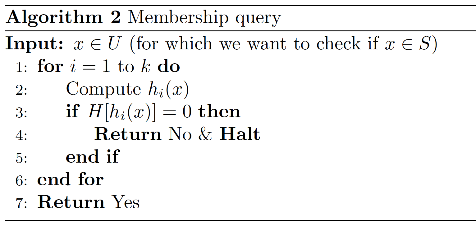
A Bloom filter maintains a 0-1 table/array \(H\) of size \(n=cm\), and uses \(k\) hash functions \(h_1,...,h_k : U \rightarrow \{ 0,1, ..., n-1 \}\). The table \(H\) is initialized to be all-zero, i.e., for each \(j =0\) to \(n-1\) we set \(H[j] = 0\).
We consider two tasks, inserting an element \(x\) into \(S\) and checking if an element \(x \in S\) or not. Deletions are not allowed.
If \(x \in S\), then Algorithm 2 outputs Yes always. Meanwhile, if \(x \notin S\), then it might incorrectly output Yes; this is called a false positive. The false positive rate is the probability of getting a false positive, i.e., the failure probability.
Our goal is to estimate the false positive rate as a function of \(k\) which is the number of hash functions used, and \(c = n/m\) which is the ratio betweeen sizes of the table \(H\) and the set \(S\). Observe that increasing \(c\) (i.e., having a larger table \(H\)) always decreases the false positive rate; however, how it depends on \(k\), the number of hash functions, is not so obvious. Our goal is to find the optimal choice of \(k\) for a given \(c\).
For any location \(j\), we have that
\[\Pr(H[j]=0) = ((1-\frac{1}{n})^k)^m = (1-\frac{1}{cm})^{km} \approx e^{-k/c},\]assuming \(m\) is large.
Suppose the input \(x\) to Algorithm 2 is not in \(S\). Then we have
\[\Pr(\text{output Yes}) = \Pr(\forall i : H[h_i(x)]=1) \approx (e^{-k/c})^k.\]Therefore, the false positive rate is approximately given by
\[f(c,k) = (e^{-k/c})^k.\]Now fix \(c\), we aim to find the optimal \(k\) which minimizes \(f(c,k)\). By calculus, the minimizer \(k\) turns out to satisfy
\[\frac{k}{c} = \log{2}.\]So we set \(k = (\log{2})c \approx 0.693c\) (or \(c \approx 1.443k\)). The false positive rate the becomes
\[\Pr(\text{false positive}) \approx (e^{-k/c})^k = \frac{1}{2^k}.\]Therefore, increasing \(k\) (i.e., using more hash functions) while maintaining \(k/c = \log{2}\) (so \(c\) is increasing at the same time) allows us to decrease the false positive rate exponentially fast, at a price of larger time and space complexity.
When \(k/c = \log{2}\), we have
\(\Pr(H[j]=0) \approx e^{-k/c} = \frac{1}{2}.\)
So \(H\) is a uniformly random 0-1 string after inserting all \(m\) elements.
Cuckoo Hashing
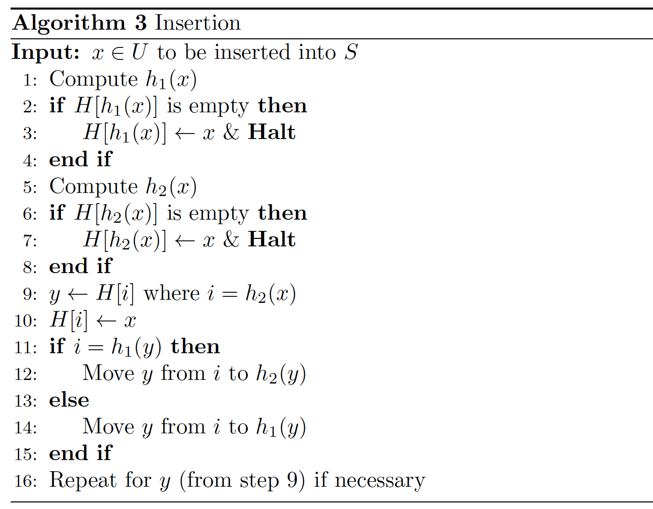
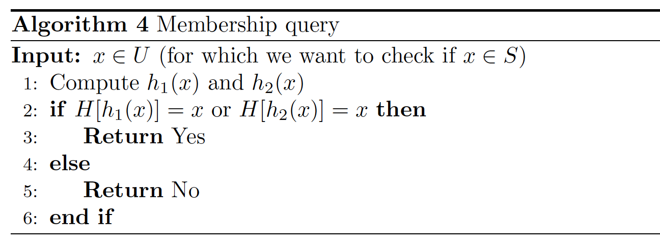
In Cuckoo hashing, we maintain a hash table \(H\) of size \(n=cm\) and use two hash functions \(h_1, h_2 : U \rightarrow \{ 0,1, ..., n-1 \}\). Each element \(x \in U\) has two possible locations \(h_1(x)\) and \(h_2(x)\) given by the hash functions. When inserting \(x\), we use whichever is empty. If neither of the locations is empty, then we add \(x\) to one of the location, say \(h_2(x)\), and move the element \(y\) previously at \(h_2(x)\) to the other possible location of \(y\).
Note that \(y\) is still at one of its possible locations \(h1(y)\) and \(h2(y)\). If the other location of \(y\) is empty, then we are done after moving \(y\) to there. Otherwise, we put \(y\) there and move the element \(z\) previously there to its other location. We will repeat this process until success.
Below shows this algorithm.
A potential problem of Algorithm 3 is the cycle of moves which causes an innite loop. If this happens, we start over with two new hash functions (rehash), and insert all elements of \(S\) from the beginning.
We observe and establish the following properties of Cuckoo hashing, assuming \(c = n/m\) is sufficiently large:
\(O(1)\) query time and no errors;
\(O(1)\) expected insertion time;
Probability of rehashing is at most 1/2.
The first property is easy to see from the algorithm design. To prove the last two properties, we need to introduce a new concept:
Definition (Cuckoo Graph). The Cuckoo graph \(G\) is a multigraph (with possibly multiple edges and self-loops) associated with the hash table \(H\) and hash functions \(h1, h2\). Vertices of \(G\) are locations/entries of \(H\), so there are \(n\) vertices. Edges of \(G\) show possible locations for all elements of S. More speci cally, for each \(x \in S\), add edge \(\{h1(x), h2(x)\}\) and label this edge by \(x\). So there are \(m\) edges.
We have the following crucial observation: If \(G\) has no cycles (i.e., \(G\) is a forest), then all \(m\) insertions succeed.
In the rest of this section, we assume that \(n \geq 6m\), i.e., \(c = n/m =6\). For any locations \(i,j\), and any element \(x \in S\), the probability that \(\{ i,j \}\) is an edge of \(G\) labeled by \(x\) is equal to \(2/n^2\) if \(i \neq j\), and \(1/n^2\) if \(i=j\).
First consider the probability of rehashing:
\[\begin{split} \Pr(\text{rehashing}) &\leq \Pr(\exists \text{ cycle in } G)\\ & \leq \sum_{l=1}^{\infty} \Pr(\exists \text{ cycle of length } l \text{ in } G)\\ & \leq \sum_{l=1}^{\infty} n^l \cdot m^l \cdot (\frac{2}{n^2})^l\\ & \leq \sum_{l=1}^{\infty} (\frac{2m}{n})^l\\ & \leq \sum_{l=1}^{\infty} (\frac{1}{3})^l = \frac{1}{2}. \end{split}\]The expected insertion time of an element \(x\) to some location \(i\) is controlled by:
\[\begin{split} \mathbb{E}[\text{length of a longest path from } i] &\leq \mathbb{E}[\text{number of a vertices connected to } i]\\ &= \sum_{j \neq i} \Pr(i \text{ and } j \text{ are connected}). \end{split}\]For any \(j \neq i\), we have
\[\begin{split} \Pr(i \text{ and } j \text{ are connected}) &\leq \sum_{l=1}^{\infty} \Pr(\exists \text{ path from } i \text{ to } j \text{ of length }l)\\ & \leq \sum_{l=1}^{\infty} n^{l-1} \cdot m^l \cdot (\frac{2}{n^2})^l\\ & \leq \frac{1}{n} \sum_{l=1}^{\infty} (\frac{2m}{n})^l\\ & \leq \frac{1}{2n}. \end{split}\]Therefore, \(\mathbb{E}[\text{length of a longest path from } i] \leq \frac{1}{2}\).


