In the last part of the previous article, we disucssed how to determine the existence of perfect matching in a bipartite graph. Today, we are gonna to propose a way to find such a perfect matching.
Moreover, we will introduce an important type of algorithm — parallel algorithm — and see how the combination of parallelism and randomness can cooperatively promote the effiency of finding the perfect matching.
Finding a Perfect Matching in Bipartite Graphs
We consider the search problem for bipartite perfect matching: Given a balanced bipartite graph \(G = (U \cup V, E)\) where \(\lvert U \rvert = \lvert V \rvert = n\), find a perfect matching of \(G\) if one exists.
Recall that we have an algorithm to test if \(G\) has a perfect matching via polynomial identity testing in the previous article: Randomized Algorithm V — Polynomial Identity Testing.
One simple idea for finding a perfect matching in \(G\) is to use the following sequential procedure:
Try an edge \(e = uv \in E\) and check if \(G \backslash \{u, v\}\) has a perfect matching or not;
if yes, add \(e\) to the output perfect matching and repeat on the smaller graph \(G \backslash \{u, v\}\);
if no, discard \(e\) and repeat on \(G \backslash e\).
Here, \(G \backslash \{u, v\}\) is a subgraph of \(G\) where we remove vertices \(u,v\) and their adjacent edges, and \(G \backslash e\) is a subgraph where we remove a single edge \(e\).
Notice that \(G \backslash e\) is not edge contraction, a concept we introduced in the previous article, denoted as \(G / e\).
We can formalize this idea into the algorithm below.
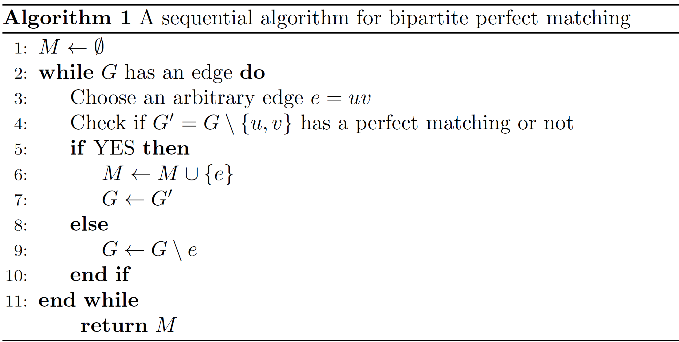
Algorithm 1 takes at most \(m = \lvert E \rvert\) rounds to find a perfect matching.
Each algorithm round requires \(O(\log{m})\) trials of bipartite perfect matching testing (with failure probability \(\leq 1/2\)), so the failure probability of each round is \(\leq 1/2m\), and by the union bound Algorithm1 fails with probability at most \(1/2\).
Next, we try to use parallel design techniques to further reduce the algorithm runtime. But no need to hurry, let’s go through some basic background about parallel algorithms first.
Sequential and Parallel Algorithms
In a sequential algorithm, a single processor compute sequentially — once through, from start to finish, without other processing executing. All the algorithms we discussed so far are sequential algorithms, and we want them to run in \(\text{poly}(n)\) time.
In a parallel algorithm, multiple processors compute simultaneously, and we want the algorithm to run in \(\text{polylog}(n)\) time with \(\text{poly}(n)\) processors.
The symbol \(\text{poly}(n)\) means “some polynomial in \(n\)”; and \(\text{polylog}(n)\) means “some polynomial in \(\log{n}\)”. Namely, \(O(\text{polylog}(n))\) is equivalent to “\(O(\log^{k}{n})\) for some constant \(k\)”.
Next, we will give three example problems to show the basic design strategy of parallel algorithm.
Ex1. Summantion
To compute \(\sum_{i=1}^{n} x_i\), a sequential algorithm takes \(O(n)\) time, while a parallel algorithm runs in \(O(\log{n})\) time with \(O(n)\) processors.
In the prallel manner, it is similar adding all elements using a binary tree.
Suppose we have 8 elements \(\{1, 2, .., 8\}\). They would be added by following steps:
- Do \(1+2\), \(3+4\), \(5+6\), and \(7+8\) in four processors.
- Do \(3 + 7\), and \(11 + 15\) in two processors.
- Do \(10 + 26\).
So this algorihm runs in \(\log{8} = 3\) steps (\(O(\log{n})\)) with \(8/2=4\) processors (\(O(n)\)).
Ex2. Matrix Multiplication
To compute \(AB\) where \(A,B \in \mathbb{Z}^{n \times n}\), a sequential algorithm runs in \(O(n^\omega)\) time where \(\omega \approx 2.37\) (currently) is the matrix multiplication exponent.
The matrix multiplication is comprised of \(n^2\) seperate summations, and each summation requires \(O(n)\) processors to run in \(O(\log{n})\) time. Based on this, we can easily get a parallel algorithm for matrix multiplication running in \(O(\log{n})\) time with \(O(n^3)\) processors.
Ex3. Matrix Determinant
To compute \(\text{det}(A)\) where \(A \in \mathbb{Z}^{n \times n}\), a sequential algorithm runs in \(O(n^\omega)\) time where \(\omega \approx 2.37\) (currently) is the matrix multiplication exponent.
There is a parallel algorithm which computes the determinant in \(O(\log^2n)\) time with \(O(n^{3.5})\) processors, see this paper. This in particular gives an efficient parallel algorithm for testing if a bipartite graph \(G\) has a perfect matching or not.
Parallel Algorithm for Bipartite Perfect Matching
In this section, we will present the most complex algorithm of the series. Skipping will have no effect on understanding the articles afterwards.
Our goal is to find a perfect matching in parallel in \(\text{polylog}(n)\) time.
A first idea is to run the sequential Algorithm 1 in parallel.
Formally, for each edge \(u_iv_j \in E\), do the following in parallel:
Check if \(G \ \{ u_i, v_j \}\) contains a perfect matching or not by checking if \(\text{det}(A_{ij} \neq 0)\) or not, where \(A_{ij}\) is the Tutte matrix \(A\) with the \(i\)‘th row and \(j\)‘th column removed;
if \(\text{det}(A_{ij} \neq 0)\), then output \(u_i v_j\).
This algorihm will output a subset of edges \(\bigcup \mathcal{PM}\), where \(\mathcal{PM}\) denotes the set of all perfect matchings of \(G\).
Let \(S = \{S_1, ..., S_n \}\) be a collection of sets, the symbol \(\bigcup S\) represents \(S_1\cup \cdots \cup S_n\).
So, if \(G\) has a unique perfect matching, then this parallel algorithm indeed works.
When there are multiple perfect matchings, we would try to isolate one of them.
Our plan is to assign random weights to edges so that \(G\) has a unique minimum weight perfect matching \(M^*\) and we can check if an edge \(e \in M^*\) or not in parallel.
The following lemma is helpful to us.
(Isolation Lemma) Let \(S_1, ..., S_n \subseteq S\) be subsets of a ground set \(S\) where \(\lvert S \rvert = m\). Each element \(x \in S\) is assigned a random weight \(w(x)\) chosen independently and u.a.r. from \(\{1,...,l \}\). For each subset \(S_i\), the weight of \(S_i\) is defined as \(w(S_i) = \sum_{x \in S_i}w(x)\). Then, we have
\[\Pr(\exists \text{ a unique } S_i \text{ of min weight}) \geq 1 - \frac{m}{l}.\]You can find the proof of this lemma on its wiki page.
For each edge \(e\), we can choose a weight \(w(e)\) independently and u.a.r. from \(\{ 1,...,2m\}\). The weight of a perfect matching \(M \in \mathcal{PM}\) is defined as \(w(M) = \sum_{e \in M} w(e)\). By the isolation lemma, if \(G\) contains a perfect matching, then with probability at least \(1/2\) there is a unique perfect matching \(M^*\) of minimum weight.
We define an \(n \times n\) matrix \(D = (d_{ij})_{i,j=1}^n\) with entries
\[d_{ij} = \begin{cases} 2^{w(e)}, & \text{if } e = u_i v_j \in E\\ 0, & \text{otherwise}. \end{cases}\]That is, \(D\) is the Tutte matrix \(A_G = A_G(x)\) evaluated at \(x_e = 2^{w(e)}, e \in E\).
Recall that
\(\text{det}(A_G) = \sum_{M \in \mathcal{PM}} \text{sgn}({\delta}_M) \prod_{e \in M} x_e.\)
Therefore, we obtain
\(\text{det}(D) = \sum_{M \in \mathcal{PM}} \text{sgn}({\delta}_M) \prod_{e \in M} 2^{w(e)} = \sum_{M \in \mathcal{PM}} \text{sgn}({\delta}_M) 2^{w(M)}.\)
Here we have two key facts about \(\text{det}(D)\): (proof omitted)
If \(G\) does not contain a perfect matching, then \(\text{det}(D) \neq 0\);
If \(G\) has a unique minimum weight perfect matching \(M^*\), then \(\text{det}(D) = 0\) and the maximum power of 2 dividing \(\text{det}(D)\) is \(w(M^*)\), i.e.,
The symbol \(m \mid n\) means “\(m\) divides \(n\)”; and \(m \nmid n\) is its “not” version. For example, \(2 \mid 10\), but \(3 \nmid 10\). See this wiki page for more information.
Finally, we can contruct the following parallel randomizzed algorithm to find the perfect matching.
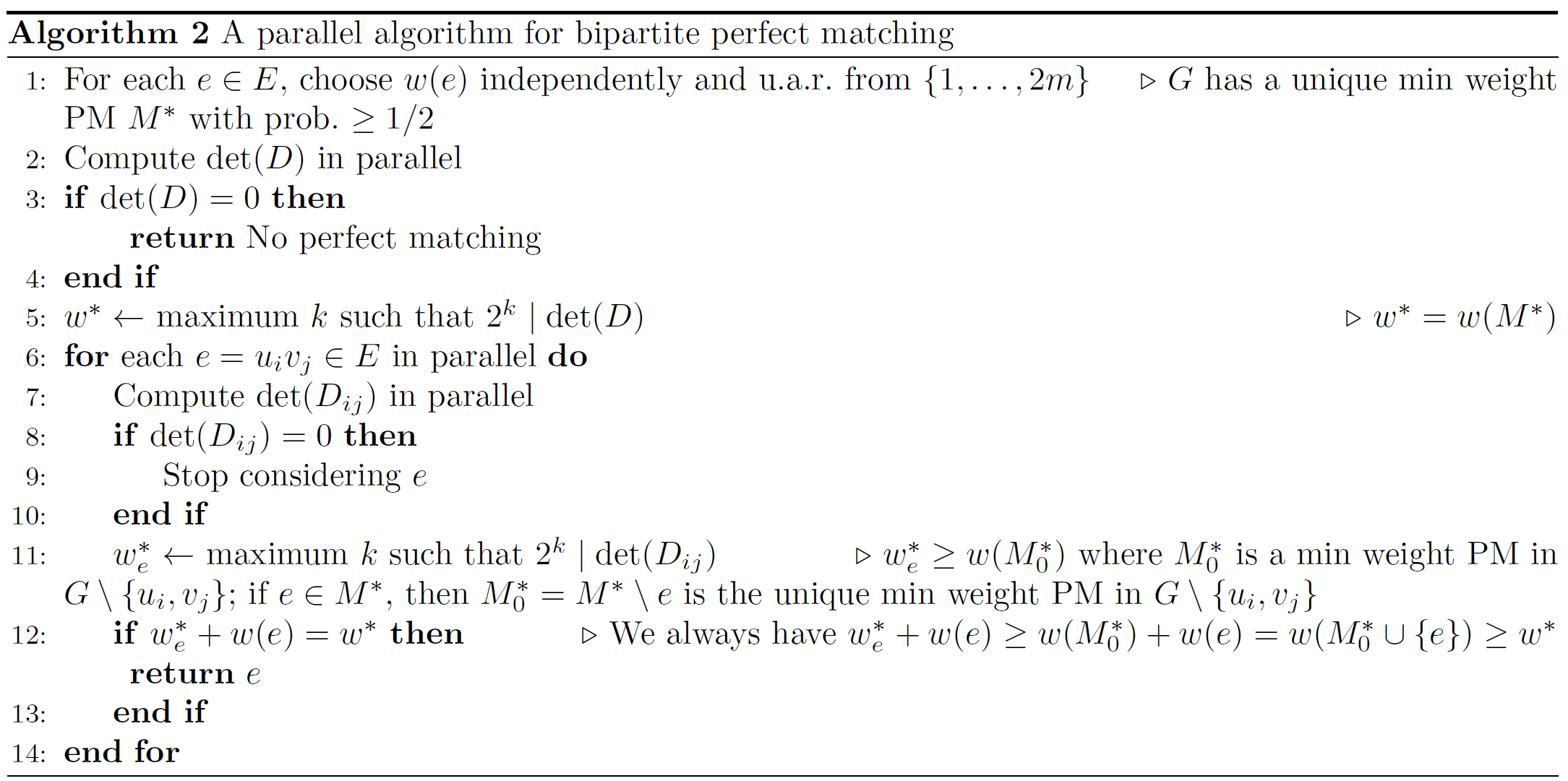
As long as the random weights of edges satisfy that \(G\) has a unique minimum weight perfect matching, Algorithm 2 successfully finds it in parallel in \(\text{polylog}(n)\) time. Thus, the success probability of Algorithm 2 is at least \(1/2\) by the isolation lemma.