Checking whether two arithmatic expressions (polynomials) are identical is one of the most important open problems in the intersection of algebra and computational complexity. Many hard problems in discrete mathematics can be smartly transformed into this class of problems. In this article, we will introduce a randomized algorithm for the polynomial identity testing (PIT) problem, and present two classical problems that can be converted to PIT and get solved.
PIT Introduction
We consider the polynomial identity testing (PIT) problem: Given two polynomial \(Q\) and \(R\) of degree at most \(d\) in \(n\) variables \(x_1, ..., x_n\), determine whether \(Q = R\) or not.
For example, following shows a polynomial of degree at most 3 and 2 variables \(x\) and \(y\).
\[Q(x, y) = x + xy + xy^2\]The question “does \((x+y)(x-y)\) equal \(x^2 - y^2\)” is a typical polynomial identity testing problem.
If we are given the polynomial as an algebraic expression (rather than as a black-box), we can confirm that the equality holds through brute-force multiplication and addition, and the time complexity of brute-force approach grows as \(C_{n+d}^{d}\). If \(n\) and \(d\) are both large, \(C_{n+d}^{d}\) grows exponentially.
Nevertheless, in many cases, we cannot even “write down” the polynomials \(Q\) and \(R\) completely or explicitly. But we are able to evaluate polynomials efficiently at any given point. In other words, given values \(x_1, ..., x_n\), we can know the value of \(Q(x_1, ..., x_n)\) and \(R(x_1, ..., x_n)\) quickly. This process is called oracle access.
Consider the polynomial \(P = Q-R\), which also has degree at most \(d\), and we can evaluate \(P\) at a given point by evaluating both \(Q\) and \(R\). Further, \(Q = R\) if and only if \(P = 0\). We thus obtain the following simpler but equivalent version of polynomial identity testing.
Polynomial identity testing problem: Given oracle access to a polynomial \(P\) of degree at most \(d\) in \(n\) variables \(x_1, ..., x_n\), determine whether \(P = 0\) or not.
Randomized Algorithm for PIT
We give a randomized algorithm as follows.
“u.a.r” means “uniformly and randomly”.
Here is a lemma about this algorithm.
(Schwartz-Zippel Lemma) For any finite set \(S\), let \(x_1,...,x_n\) be selected independently and u.a.r from \(S\), if \(P \neq 0\), then
\[\Pr(P(x_1,...,x_n) = 0) \leq \frac{d}{|S|} \text{.}\]You can find a proof of this lemma here.
In our algorihm, we choose \(\lvert S \rvert = 2d\), so by this lemma, we obtain the success and failure probailities as summarized in the table below.
| Pr(return YES) | Pr(return NO) | |
|---|---|---|
| \(P=0\) | 1 | 0 |
| \(P \neq 0\) | \(\leq \frac{1}{2}\) | \(\geq \frac{1}{2}\) |
Next, we will give two examples to illustrate the application of PIT problem - matrix multiplication testing and bipartite perfect matching.
Matrix Multiplication Testing
Recall the matrix mutiplication testing problem we disucssed in the first article of this series (Randomized Algorithm I — Introduction): Given three matrices \(A, B. C \in \mathbb{Z}^{n \times n}\), determine whether \(AB = C\) or not.
Consider \(n\) polynomials of degree at most 1 (i.e., linear functions) in \(n\) variables \(x_1, ..., x_n\) given by
\[P (x_1, ..., x_n) = \begin{pmatrix} P_1 (x_1, ..., x_n)\\ \vdots \\ P_n (x_1, ..., x_n) \end{pmatrix} = (AB-C) \begin{pmatrix} x_1\\ \vdots \\ x_n \end{pmatrix} \text{.}\]Each polynomial \(P_i\) has degree at most 1. Futhermore, given values \(x_1, ..., x_n\), we can evaluate \(P(x_1, ..., x_n)\) in \(O(n^2)\) time since \((AB-C)x = A(Bx) - Cx\).
Observe that \(AB = C\) if and only if \(P = 0\), i.e., \(P_1=\cdots = P_n = 0\). Therefore, our randomized algorithm for PIT covers Freivald’s algorithm for matrix multiplication testing.
Bipartite Perfect Matching
Problem Description
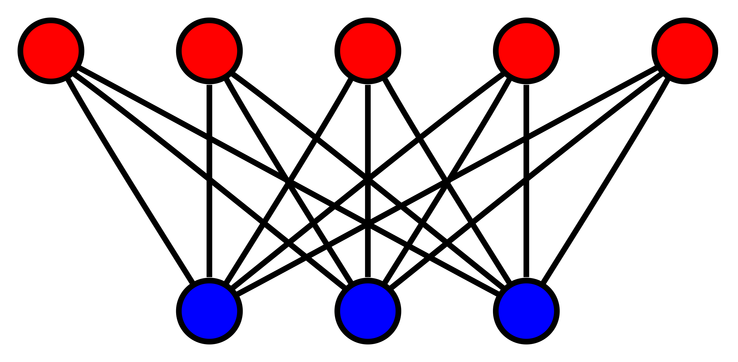
Given a bipartite graph \(G = (U \cup V, E)\) where \(\lvert U \rvert = \lvert V \rvert = n\) (balanced bipartite graph), we want to determine whether or not \(G\) has a perfect matching.
Here are two new concepts:
- Bipartite graph: a graph \(G = (V, E)\) is bipartite if and only if \(V\) can be partitioned into two non-empty subsets \(U\) and \(V\), such that every edge in \(E\) has one endpoint in \(U\) and the other endpoint in \(V\).
Following is a bipartite graph.
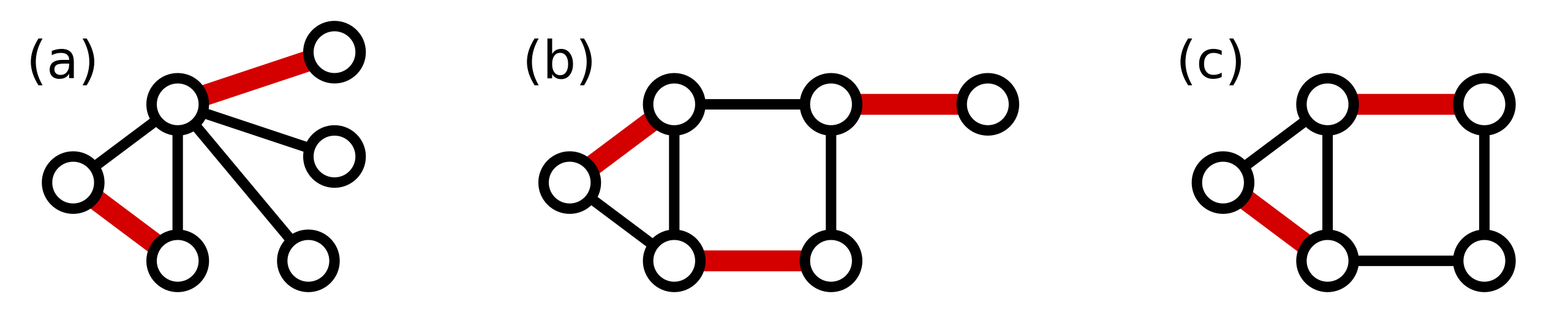
- Perfect mathcing: given a graph \(G = (V, E)\), a perfect matching in \(G\) is a edge subset \(M \subseteq E\), such that every vertex in \(V\) is adjacent to exactly one edge in \(M\).
In the following three graphs, only (b) has a perfect matching.
The bipartite perfect matching problem has many real applications. For example, in a job market, the relationship between employers and job seekers can be depicted using a bipartite graph. The existence of the perfect matching determines whether every job seeker could be assigned to a suitable job.
Tutte Matrix & Lemma
For a bipartite graph \(G = (U \cup V, E)\), where \(U = (u1, ..., u_n)\) and \(V = {v_1, ..., v_n}\), the Tutte matrix of G is an \(n \times n\) matrix \(A_G = (a_{ij})_{i,j=1}^{n}\) with entries given by
\[a_{ij} = \begin{cases} x_{e}, & \text{if } e = u_i v_j \in E\\ 0, & \text{otherwise}. \end{cases}\]where the $x_e$’s are indeterminates (variables).
Here is a key lemma connecting Tutte matrix with perfect matching.
(Lemma) A balanced bipartite graph \(G\) contains a perfect matching if and only if \(\text{det}(A_G) \neq 0\), where \(\text{det}(A_G)\) is given by
\[\text{det}(A_G) = \sum_{\sigma \in S_n} \text{sgn}(\sigma) \prod_{i=1}^{n} a_{i, \sigma(i)},\]The symbol \(\text{det}(A_G)\) means the determinant of \(A_G\). Determinant is a quite complicated concept that we don’t need to understand here. You can refer to its wiki page for more information.
In the determinant expression, \(S_n\) is the set of \(n!\) permutations of \(\{1, .., n\}\); \(\text{sgn}(\sigma) \in \{ \pm 1 \}\) is the sign of a permutation \(\sigma\) given by \(\text{sgn}(\sigma) = (-1)^{\text{# of inversions in } \sigma}\); and \(\sigma(i)\) is the \(i\)‘th element in \(\sigma\).
For example, if take \(n=4\) and let \(\sigma = (1,4,2,3)\) be one possible permutation, we can know that \(\sigma(2) = 4\) and \(\text{sgn}(\sigma) = 1\) because there are 2 inversions in \(\sigma\): \((4,2)\) and \((4,3)\).
We can evaluate \(\text{det}(A_G)\) in \(O(n^\omega)\) time where \(\omega \approx 2.37\) (currently) is the matrix multiplication exponent.
Observe that \(\text{det}(A_G)\) is a polynomial of degree at most \(n\) in \(m\) variables \(\{ x_e : e \in E \}\). Therefore, by the above lemma, we can use the algorithm for PIT to determine if \(G\) has a perfect matching or not.