Randomized Algorithm IV— Integer Programming

Integer programming is a type of optimization problem where the goal is to find the best integer solution to a problem.

Integer programming is a powerful problem-solving tool used in many research fields. Its potential applications range from resource allocation decisions to scheduling problems. This article will provide an overview of integer programming, outlining its fundamentals and exploring how it can be applied in algorithm tasks by applying it on the congestion minimization problem.

Integer Programming and Linear Programming

In an IP (Integer Programming) problem, we want to find an integral point that maximizes or minimizes a linear objective function under a few linear constraints.

Let $A\in {\mathbb{R}}^{m\times n}$, $b\in {\mathbb{R}}^m$, and $c\in {\mathbb{R}}^n$. In the matrix form, the objective function of IP can be written as follow. ($c^{\mathrm{T}}$ denotes the transpose of $c$.)

$$\underset{x\in {\mathbb{Z}}^n}{max}{c}^{\mathrm{T}}x\text{,}$$

which is subject to the following constraints:

$$\begin{array}{rl}Ax& \le b\\ x& \ge 0\end{array}$$

If $x$ is further restricted to $\{0,1{\}}^n$, then it is called a 0/1 IP problem.

Below shows an example of 0/1 IP problem.

$$\text{Maximize }8x_1+11x_2+6x_3$$ $$\begin{array}{rl}\text{subject to }& 5x_1+7x_2+4x_3\le 14\\ & x_1,x_2,x_3\in \{0,1\}\end{array}$$

In an LP (Linear Programming) problem, the point we want to find is not restricted to be integral. Namely, $x_i$ can be any positive real number.

An important thing to know it that: LP can be solved in polynomial time. Examples of algorithms for LP include the simplex algorithm and the ellipsoid algorithm; however, IP is NP-complete.

Congestion Minimization Problem

Problem Description

Traffic congestion occurs when a volume of traffic generates demand for space greater than the available street capacity. Given a traffic route map, for a series of trips with given starting and ending points, we need to properly arrange the routes of each trip so that they are spatially staggered as much as possible to reduce congestion on the road.

We can use a directed graph $G=(V,E)$ to model the traffic route map and $k$ source-sink pairs $(s_1,t_1),...,(s_k,t_k)$ to model trips waiting to be arranged. Our goal is to find $k$ paths $p_1,...,p_k$ where each $p_i$ is from $s_i$ to $t_i$, such that the congestion of these paths is minimized. Here, for each edge $e$ in the graph, we define its congestion as the number of paths using $e$. Formally put,

$$\text{cong}(e)=|\{i\in [k]:e\in p_i\}|\text{.}$$

$i\in [k]$ is equivalent to $i\in \{1,2,...,k\}$.

The congestion of our arrangement for all trips (paths) is defined by

$$\text{congestion}=\underset{e\in E}{max}\text{cong}(e)\text{.}$$

To minimize this congestion, next, we will turn this problem into the IP description format.

IP Description

Let ${\mathcal{P}}_i$ denote the set of all possible paths from $s_i$ to $t_i$ for every $i\in [k]$. For each path $p\in \bigcup _{i=1}^k{\mathcal{P}}_i$, let $x_p$ be an indicator variable such that $x_p=1$ if the path $p$ is used and $x_p=0$ otherwise.

Let $W\in {\mathbb{N}}^{+}$ denote the congestion of paths that we want to minimize. The congestion minimization problem can be solved by the following IP.

$$\text{min }W$$

subject to

$$\begin{array}{rl}\sum _{p\in {\mathcal{P}}_i}{x}_p=1& ,\mathrm{\forall }i\in [k]\\ \sum _{i=1}^k\sum _{p\in {\mathcal{P}}_i:e\in p}{x}_p\le W& ,\mathrm{\forall }e\in E\\ x_p\in \{0,1\}& ,\mathrm{\forall }p\in \bigcup _{i=1}^k{\mathcal{P}}_i\\ W& \in {\mathbb{N}}^{+}\end{array}$$

Solving this IP is computationally hard.

Hence, we adopt the following strategy, which is a common approach in the design of approximation aglorithm.

1. Relaxation: Solve an LP relaxation of the IP by removing the integral constraint, and obtain an optimal fractional solution;

2. Rounding: Transform the fractional solution we get into the integral solution of the original IP, and hope that it solves the IP approximately.

In general, IP is hard to solve. So, the high-level idea here is to transform IP into LP, and use the LP result (which can be got in polynomial time) to estimate the IP result.

Here, we suppose that we have a good algorithm to solve the LP problem. In the next two sections, let’s take look at the details about the relaxtion and rounding process.

LP Relaxtion

We relax the integral constraints $x_p\in \{0,1\}$ to $x_p\in [0,1]$ and $W\in {\mathbb{N}}^{+}$ to $W\ge 1$.

Let $(x_{OPT}^{IP},W_{OPT}^{IP})$ denote an optimal (integral) solution to the IP for congestion minimization, and let $(x_{OPT}^{LP},W_{OPT}^{LP})$ denote an optimal (integral) solution to the LP relaxtion. Then we have:

$$W_{OPT}^{IP}\ge W_{OPT}^{LP}$$

Simply speaking, this inequality holds because the solution set of IP is the subset of the solution set of LP relataxtion (fractional numbers include integral numbers), and as a result, LP relataxtion can achieve better optimization.

Randomized Rounding

Here, we write $(x,W)=(x_{OPT}^{LP},W_{OPT}^{LP})$ for simplicity. Our randomized rounding algorihtm is given below.

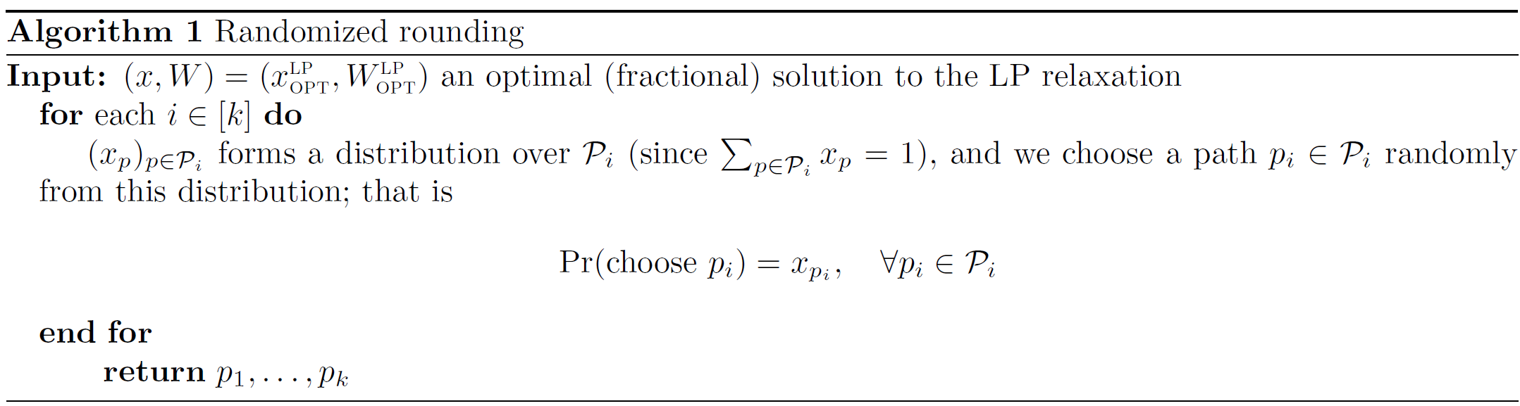
Consider that $x_p$ is a fractional value between 0 and 1, the idea of this algorithm is to regard $x_p$ as a possibility. And we use this possibility to guide the path choosing - path with larger $x_p$ has higher chance to be chosen.

Here is a key lemma, described as follows.

For every edge $e\in E$, we have

$$Pr(\text{cong}(e)\ge \frac{C\log n}{\log \log n}W)\le \frac{1}{2n^2}\text{,}$$

where $C>0$ is a large absolute constant.

The proof of this lemma is in the end of this article.

Given this lemma, we are able to bound the congestion of paths we get via randomized rounding. Recall that $\text{congestion}=\underset{e\in E}{max}\text{cong}(e)$. We deduce that

$$\begin{array}{rl}Pr(\text{congestion}\ge \frac{C\log n}{\log \log n}{W}_{OPT}^{IP})& \le Pr(\text{congestion}\ge \frac{C\log n}{\log \log n}{W}_{OPT}^{LP})\\ & \le \sum _{e\in E}Pr(\text{cong}(e)\ge \frac{C\log n}{\log \log n}W)\\ & \le |E|\cdot \frac{1}{2n^2}\le \frac{1}{2}\end{array}$$

The first inequality comes from the fact in the LP Relaxtion section; the second inequality is union bound; the third inequality uses the above lemma.

Therefore, with probability at least $1/2$, the congestion of paths we find is at most $\frac{C\log n}{\log \log n}$ times minimum congestion.

In other words, we can achieve an approximation ratio of $\frac{C\log n}{\log \log n}$ with high probability.

Proof

This section is optional to read.

In this section, let’s prove the lemma presented in the Randomized Rounding section.

Before we start, a special version of Chernoff bounds, which is suitable when the deviation is large, has to be introduced.

(Chernoff bounds) Let $X_1,...,X_n$ be independent random variables taking values in [0, 1]. Let $X=\sum _{i=1}^n{X}_i$ be their sum with mean $\mu =\mathbb{E}X=\sum _{i=1}^{n}E{X}_i$. Then we have:

$$\mathrm{\forall }\delta \ge 0:Pr(X\ge (1+\delta )\mu )\le (\frac{e^{\delta }}{(1+\delta {)}^{1+\delta }}{)}^{\mu }\le (\frac{e}{1+\delta }{)}^{(1+\delta )\mu }\text{;}$$ $$\text{Equivalently, }\mathrm{\forall }a\ge \mu :Pr(X\ge a)\le (\frac{e\mu }{a}{)}^a\text{.}$$

Following is the proof of the lemma.

Let $X_i$ be an indicator random variable such that $X_i=1$ if $e\in p_i$ and $X_i=0$ otherwise. Note that $X_1,...,X_k$ are jointly independent. Then we have

$$X=\sum _{i=1}^k{X}_i=\text{cong}(e)\text{.}$$

Notice that

$$\mathbb{E}{X}_i=Pr(e\in p_i)=\sum _{p_i\in {\mathcal{P}}_i:e\in p_i}Pr(\text{choose }{p}_i)=\sum _{p_i\in {\mathcal{P}}_i:e\in p_i}{x}_{p_i}\text{.}$$

Therefore, by the constraint of LP we have

$$\mathbb{E}X=\sum _{i=1}^k\mathbb{E}{X}_i=\sum _{i=1}^k\sum _{p_i\in {\mathcal{P}}_i:e\in p_i}{x}_{p_i}\le W\text{.}$$

We deduce from the Chernoff bound that

$$\begin{array}{rl}Pr(X\ge \frac{C\log n}{\log \log n}W)& \le (\frac{e\mathbb{E}X}{\frac{C\log n}{\log \log n}W}{)}^{\frac{C\log n}{\log \log n}W}\\ & \le (\frac{\log \log n}{\log n}{)}^{\frac{C\log n}{\log \log n}}(\mathbb{E}X\le W,e\le C,W\ge 1)\\ & \le (\frac{1}{\sqrt{\log n}}{)}^{\frac{C\log n}{\log \log n}}(\log \log n\le \sqrt{\log n}\text{ when }n\text{ is sufficiently large})\\ & =e^{-\frac{1}{2}\log \log n\cdot \frac{C\log n}{\log \log n}}\le \frac{1}{2n^2}\text{,}\end{array}$$

where $C>0$ is a large constant independent of $n$.