In this article, we will introduce three important inequalities for possibility concentration. Then, we provide an example problem - Mean Estimation - to show the application of Chernoff bound.
Inequalities
Markov’s Inequiality
Let \(X\) be a non-negative random variable with mean \(\mu = \mathbb{E}X\). Then we have:
\[\begin{split} \forall a \geq 0&: \Pr(X \geq a \mu) \leq \frac{1}{a} \\ \text{Equivalently, } \forall a \geq 0&: \Pr(X \geq a) \leq \frac{\mu}{a} \end{split}\]Chebyshev’s Inequality
Let \(X\) be a non-negative random variable with mean \(\mu = \mathbb{E}X\) and variance \(\delta^2 = \text{Var}(X)\). Then we have:
\[\begin{split} \forall a \geq 0&: \Pr(|X-\mu| \geq a \delta) \leq \frac{1}{a^2} \\ \text{Equivalently, } \forall a \geq 0&: \Pr(|X-\mu| \geq a) \leq \frac{\delta^2}{a^2} \end{split}\]Chernoff Bounds
Let \(X_1, ..., X_n\) be independent random variables taking values in [0, 1]. Let \(X = \sum_{i=1}^{n}X_i\) be their sum with mean \(\mu = \mathbb{E}X = \sum_{i=1}^{n}{E}X_i\). Then we have:
\[\begin{split} \forall \delta \geq 0: \Pr(X \geq (1+\delta) \mu) &\leq (\frac{e^\delta}{(1+\delta)^{1+\delta}})^\mu \\ and \quad \Pr(X \leq (1-\delta) \mu) &\leq (\frac{e^{-\delta}}{(1-\delta)^{1-\delta}})^\mu \end{split}\]A looser but simpler version (also more useful in practice) is:
\[\begin{split}\forall \delta \in (0,1): \Pr(X \geq (1+\delta) \mu) &\leq e^{-\frac{\delta^2 \mu}{3}} \\ and \quad \Pr(X \leq (1-\delta) \mu) &\leq e^{-\frac{\delta^2 \mu}{2}} \end{split}\]Mean Estimation
Problem Description
Suppose \(X_1, X_2, ...\) are i.i.d. (independent and identically distributed) of a random variable \(X\). Our goal is to estimate \(\mathbb{E}X\) from these samples. Moreover, we want to understand how many samples are needed so that our estimate \(\hat{X}\) satisfies
\[\Pr(|\hat{X} - \mathbb{E}X| \leq \varepsilon \mathbb{E}X) \geq 1- \delta \text{,}\]where \(\varepsilon, \delta \in (0,1)\) are given. Here \(\varepsilon\) is the approximation error and \(\delta\) is the failure probability.
Simple Approach: Sample Mean
Suppose we have \(n\) i.i.d. samples \(X_1, ..., X_n\). Let \(Y = \sum_{i=1}^{n}X_i\) be their sum, so \(\mathbb{E}Y = n\mathbb{E}X\). Let \(\hat{X} = Y / n\) be the sample mean, so \(\mathbb{E}X = \mathbb{E}\hat{X}\). We have
\[\Pr(|\hat{X} - \mathbb{E}X| \geq \varepsilon \mathbb{E}X) = \Pr(|Y - \mathbb{E}X| \geq \varepsilon \mathbb{E}X)\]We cannot use the Chernoff bound here since \(X\) may not be bounded (e.g., \(X\) is geometric or Gaussian). Instead, we apply the Chebyshev’s inequality:
\[\Pr(|Y - \mathbb{E}X| \geq \varepsilon \mathbb{E}X) \leq \frac{\text{Var}(Y)}{(\varepsilon \mathbb{E}Y)^2} = \frac{n\text{Var}(X)}{(\varepsilon n\mathbb{E}X)^2} = \frac{r^2}{\varepsilon^2 n} \text{,}\]where
\[r = \frac{\sqrt{\text{Var}(X)}}{\mathbb{E}X} \text{.}\]We want the failure probability to be at most \(\delta\), so it suffices to take
\[\frac{r^2}{\varepsilon^2 n} \leq \delta \Longleftrightarrow n \geq \frac{r^2}{\varepsilon^2 \delta} \text{.}\]Based on this result, we can know that the number of samples we need is \(n = O(r^2 / (\varepsilon^2 \delta))\). The linear dependency on \(1/\delta\) is bad for many applications. In the next section, we will give a better approach which achieves \(\log(1/\delta)\) dependency for sample complexity.
Better Approach: Median of Means
Assume we choose \(m = 4r^2/\varepsilon^2\) samples and calculate the esimate \(\hat{X} = \frac{1}{m} \sum_{i=1}^{m}X_i\), we have:
\[\Pr(|\hat{X} - \mathbb{E}X| \geq \varepsilon \mathbb{E}X) \leq \frac{r^2}{\varepsilon^2m} = \frac{1}{4}\]We say \(\hat{X}\) is a good estimation if \(\lvert \hat{X} - \mathbb{E}X \rvert \leq \varepsilon \mathbb{E}X\). Therefore, \(\Pr(\hat{X} \text{ is good}) \geq 3/4\).
Our plan is to generate many such estimates \(\hat{X}\) independently. Since each estimate is good with probability at least 3/4, the majority of these estimates would be good with high probability, and hence we can use the median of these estimates as our final estimator. We can formalize our idea into the following “Median of Means” algorithm.
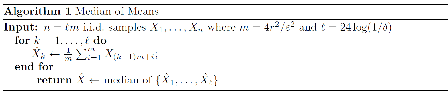
The idea of this algorithm is to take means first and then take median of means as the final estimation. Using this algorithm, the number of samples we need is
\[n = lm =24\log{1/\delta} \cdot \frac{4r^2}{\varepsilon^2} = O(\frac{r2}{\varepsilon^2}log(1/\delta)) \text{.}\]So, this approach indeed achieves \(\log(1/\delta)\) dependency for sample complexity. Good job!
In the rest part of this section, if you still have energy, let’s look at why taking \(l = 24\log(1/\delta)\) can ensure the estimation has high possibility to be good.
We know that \(\hat{X}_1, ..., \hat{X}_l\) are jointly independent. For each \(k\), we have \(\Pr(\hat{X}_k \text{ is good}) \geq 3/4\). To faciliate follow-up mathematical processing, we define \(Z_k\) to be a Bernoulli random variable such that \(Z_k = 1\) if \(\hat{X}_k\) is good, and \(Z_k = 0\) otherwise. Let \(Z = \sum_{k=1}^{l} Z_k\) be the number of good estimates among all \(l\) of them.
Note that \(Z_1, ..., Z_k\) are independent and \(\mathbb{E}Z_k = \Pr(\hat{X}_k \text{ is good}) \geq 3/4\). Hence, \(\mathbb{E}Z \geq 3l/4\).
Here comes a key observation:
If more than half of the estimates in \(\{ \hat{X}_1, ..., \hat{X}_l \}\) are good, then the median \(\hat{X}\) of them is good.
Based on this, we have:
\[\Pr(\hat{X} \text{ is not good}) \leq \Pr(Z \leq \frac{l}{2}) \leq \Pr(Z \leq \frac{2}{3} \mathbb{E}Z)\]Now we can apply the looser version of Chernoff Bound:
\[\Pr(Z \leq \frac{2}{3} \mathbb{E}Z) \leq e^{-\frac{(1/3)^2\mathbb{E}Z}{2}} \leq e^{-\frac{(1/3)^2(3l/4)}{2}} = e^{-l/24}\]To make the failure probability at most \(\delta\), it suffices to take
\[e^{-l/24} \leq \delta \Longleftrightarrow l \geq 24 \log{1/\delta} \text{.}\]As a result, when \(l \geq 24 \log{1/\delta}\), we have \(\Pr(\hat{X} \text{ is good}) \geq 1-\delta\).