Randomized Algorithm II — Global Min Cut & Median

In this article, we discuss two typical and educational problems which can be well solved using randomized algorithm - global min cut problem and median problem.

Global Min Cut

Problem Background

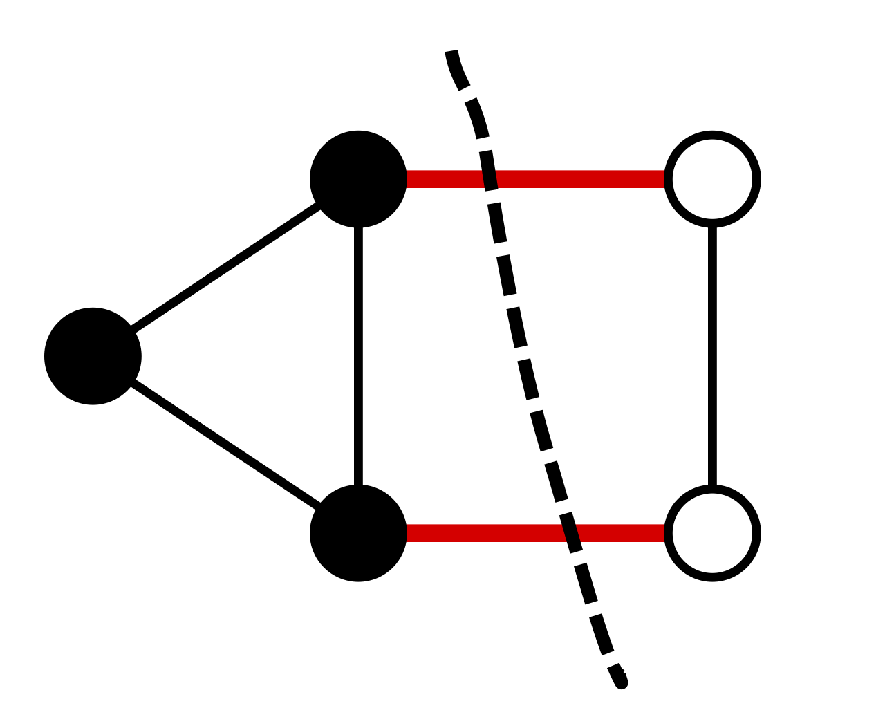
In graph theory, a cut is a partition of the vertices of a graph into two disjoint subsets. The size of a cut is defind as the number of edges across two partitions. A cut is minimum if the size of the cut is not larger than the size of any other cut. The illustration below shows a minimum cut: the size of this cut is 2.

The gloabl min cut problem is how to find the minimum cut in a given graph. A closely related problem is the min s-t cut problem, where two extral vertices s and t are provided. In the min s-t cut problem, we require s and t are divided by the cut. In other words, s should be in one vertex partition, and t should be in another.

One can solve the min s-t cut problem using any polynomial-time algorithm for max s-t flow, and the current fastest algorithm runs in $O(m^{1+o(1)})$ time. Hence, a naive strategy is to divide the global min cut problem to $n-1$ min s-t cut problems: If the graph vertex set $V=\{v_1,...,v_n\}$, then we solve min $v_1$ - $v_i$ cut for each $i=2,...,n$ and output the best cut among these $n-1$ cuts.

Karger’s Algorithm

Here we only consider multigraphs without self-loops, i.e., there are possibly multiple edges between a pair of distinct vertices but no edges linking to itself. Following is the randomized algorithm to find the global min cut.

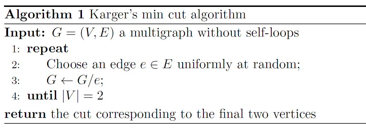
In each loop, this algorithm randomly choose an edge from the graph, and do the edge contraction in line 3. During the edge contraction operation ($G/e$), The edge $e$ is removed and its two incident vertices, $u$ and $v$, are merged into a new vertex, as illustrated below.

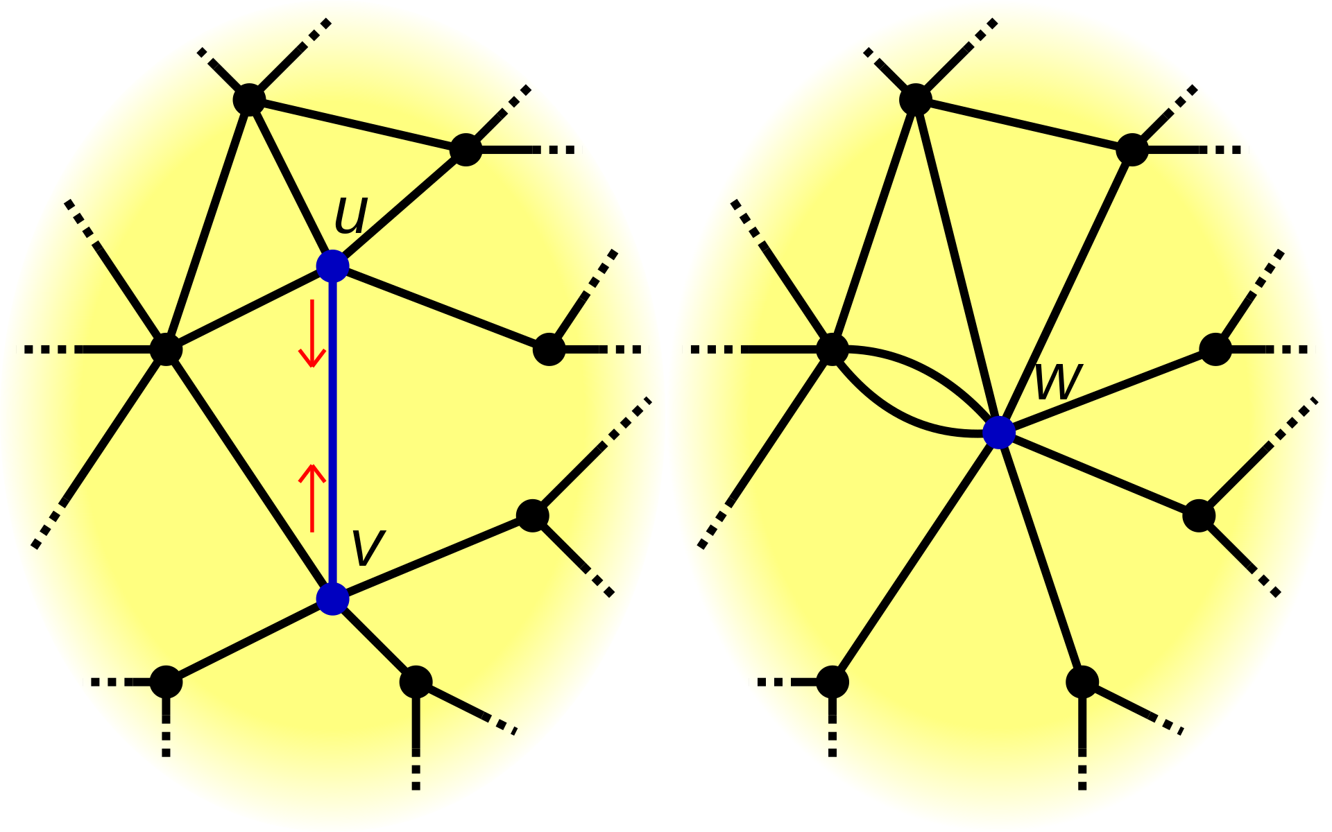
Note that after each edge contraction, the new graph is still a multigraph without self-loops.

If you remain confusion about the edge contraction after view the above picture, we provide a formal definition here. We define $G/e$ to be the graph resulted from contraction of $e$ by:

1. Replace $u,v$ by a new vertex $w$;
2. Replace every edge $ux$ or $vx$ where $x\in V\mathrm{\setminus }\{u,v\}$ by a new edge $wx$.

The algorithm ends when there are only two vertices left in the graph, and output the number of edges between them.

In fact, the edge contraction process is partitioning the original vertex set, and the edges between last two vertices represent the cut of this partition.

Here is a lemma describing the success possibility of this algorithm:

$$Pr(\text{Algorithm1 outputs the global min cut})\ge \frac{1}{C_n^2}$$

The proof of this lemma is at the end of this article.

As we did before, we can boost the success possibility by multiple runs. Here, if we run this algorithm for $C_n^2\cdot c\log n$ times where $c>0$ is some constant, and output the best cut among them. Then we have:

$$\begin{gathered} Pr(\text{none of these runs output the global min cut}) \\ \le (1-\frac{1}{C_n^2}{)}^{C_n^2\cdot c\log n}\le e^{-c\log n}=\frac{1}{n^c} \end{gathered}$$

The first inequality we used here is union bound, which says that for a set of events, the probability that at least one of the events happens is no greater than the sum of the probabilities of the individual events; the second inequality is $(1+\frac{1}{k}{)}^k\le e$, which is an extended form of Bernoulli’s inequality. These two inequalities are extremely useful in the possibility bounding of randomized algorithm.

So, the success possibility after multiple runs is at least $1-1/n^c$. This means that to guarantee a success probability at least $1-1/\text{ploy}(n)$, it suffices to run the algorithm for $O(n^2\log n)$ times.

Finally, let’s look at the overall running time. If we use the adjacency matrix representation, every edge contraction takes $O(n)$ time. Thus, each run of the algorithm takes $O(n^2)$ time. The overall running time to get success probability at least $1-1/\text{ploy}(n)$ is $O(n^4\log n)$. Such running time is even slower than the naive solution we provided in the Introduction section. Next, we will discuss how to improve this randomized algorithm.

Karger-Stein Algorithm

First, let’s examine the possibility of global min cut surviving when only $l$ vertices are left in the Karger’s Algorithm, meaning that all of the first selected $n-l$ edges do not belong to the min cut. Suppse $e_i$ represents the i-th selected edge ($i\ge 0$), then we have: (calculation is omitted)

$$Pr(\text{global min cut survives down to }l\text{ vertices})=Pr(e_0,e_1,...,e_{n-l-1}\notin \text{global min cut})\ge \frac{C_l^2}{C_n^2}$$

Looking close to this inequality, we will find the lower bound of surviving possibility is close to one in initial loops. For example, after the first loop, where $l=n-1$, the possibility is at least $1-2/n$. However, this value drops faster and faster when $l$ decreases from $n$ to $2$. In other words, in the Karger’s Algorithm, initial edge contractions are likely correct, while later edge contractions are much less likely to be correct. Thus, instead of running the whole Algorithm 1 for multiple times, a better way is to run initial edge contractions fewer times while later contractions more times.

We can observe that when $l\approx n/\sqrt{2}$, the possibility is at least $1/2$. Based on this, the algorithm can be modified into such resursive style:

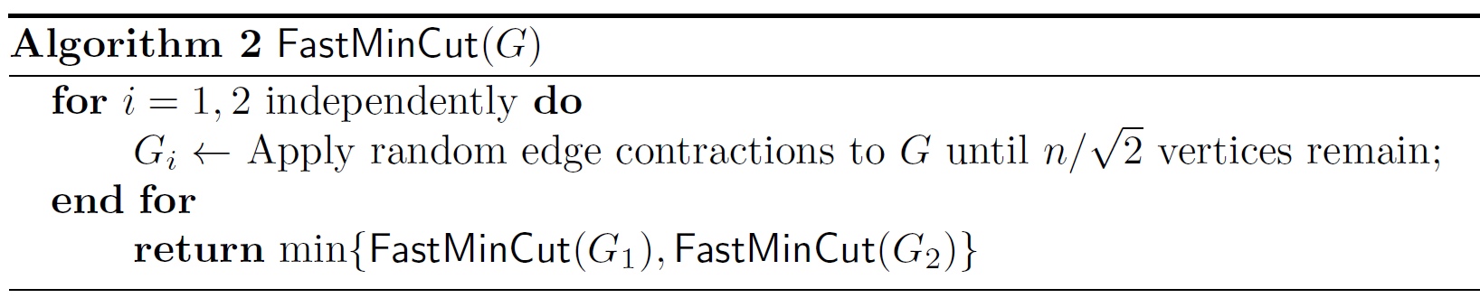
Defind $P(n)$ to be the probability of success of Algorithm 2 on any n-vertex graph. We have the recursion:

$$1-P(n)\le (1-\frac{1}{2}P(\frac{n}{\sqrt{2}}){)}^2$$

Solving the recursion gives $P(n)=\mathrm{\Omega }(1/\log n)$.

The running time of Algorithm2 satisfies the recursion:

$$T(n)=2T(\frac{n}{\sqrt{2}})+O(n^2)$$

Therefore, $T(n)=O(n^2\log n)$. To get success probability at least $1-1/\text{ploy}(n)$, we run Algorithm2 for $O({\log }^{2}n)$ times and the overall running time is $O(n^2{\log }^{3}n)$.

Median

In this section, let’s disucss a easier one - the median problem, which is described as this: Given an unsorted list $S=[s_1,...,s_n]$ of integers, find the median of them. A straight-forward way to find the median is to sort them first, taking $O(n\log n)$ time, and then output the value we want.

QuickSelect is a simple randomized algorithm with expected running time $O(n)$. The approach is described as follow.

1. Find a good “pivot” $p\in S$;
2. Partition $S$ into $S_{\le p}=\{x\in S:x\le p\}$ and $S_{>p}=\{x\in S:x>p\}$;
3. The median is in one of $S_{\le p}$ and $S_{>p}$, and recurse.

We say the pivot $p$ is good if both $S_{\le p}\le 3n/4$ and $S_{>p}\le 3n/4$. This means that a good pivot should be close to the median. Assume that we always get a good pivot, the running time of QuickSelect then satisfies the recursion:

$$T(n)=T(\frac{3n}{4})+O(n)$$

Solving the recursion gives $T(n)=O(n)$.

Here we introduce a simple strategy to find good pivots - picking random elements from $S$. According to our definition about good pivot, $p$ is good if it is in between the ($n/4$)th smallest element and the ($3n/4$)th smallest element. Hence, there are (at least) $n/2$ good pivots, indicating that with $1/2$ possibility we can find a good pivot by randomly picking.

Knowing this, we can follow such a procedure to find a good pivot: Choose a random pivot and check if it is good; if not, repeat. The number of rounds needed to find a good one is $O(1)$ in expectation (beacuse it is in geometry distribution). As a result, the overall running time of QuickSelect is in $O(n)$ expectation.

Checking whether a pivot $p$ is good is equivalent to checking whether $S_{\le p}\le 3n/4$ and $S_{>p}\le 3n/4$, which takes $O(n)$ time.

Conclusion

After going through these two basic problems, you may find that the design of randomized algorithm is not as complicated as normal algorithms. All the algorithms we discussed in this article are not longer than four lines! The intricate thing is to decide how many runs are neeeded to boost the success possibility to the $1-1/\text{ploy}(n)$ level.

“Success possibility at least $1-1/\text{ploy}(n)$” is a de facto standard in the theory field.

Proof

This section is optional to read.

Given $G=(V,E)$ as a multigraph without self-loops. Suppose a vertex bipartition $(S^{\ast },V\mathrm{\setminus }{S}^{\ast })$ is a global min cut of $G$, where $S^{\ast }\subseteq V$. Let ${\delta }^{\ast }$ denote the edge set of global min cut of $G$. Namely,

$${\delta }^{\ast }=E(S^{\ast },V\mathrm{\setminus }{S}^{\ast })=\{uv\in E:u\in S^{\ast },v\in V\mathrm{\setminus }{S}^{\ast }\}$$

Let’s prove the lemma:

$$Pr(\text{Algorithm1 outputs }{\delta }^{\ast })\ge \frac{1}{C_n^2}\text{.}$$

Denote the sequence of edges chosen and contracted by Algorithm 1 as $e_0,e_1,...,e_{n-3}$; note that we need to contract $n-2$ edges to get down to two vertices.

A key observation here is that Algorithm 1 outputs ${\delta }^{\ast }$ if and only if $e_0,e_1,...,e_{n-3}\notin {\delta }^{\ast }$. This means that each edge chosen to be contracted is inside of $S^{\ast }$ or $V\mathrm{\setminus }{S}^{\ast }$. No chosen edge is across these two vertex sets. So, we have

$$Pr(\text{Algorithm1 outputs }{\delta }^{\ast })=Pr(e_0,e_1,...,e_{n-3}\notin {\delta }^{\ast })$$

By the chain rule, we have

$$\begin{array}{rl}& Pr(e_0,e_1,...,e_{n-3}\notin {\delta }^{\ast })\\ =& Pr(e_0\notin {\delta }^{\ast })Pr(e_1\notin {\delta }^{\ast }|e_0\notin {\delta }^{\ast })Pr(e_2\notin {\delta }^{\ast }|e_0,e_1\notin {\delta }^{\ast })\\ & \cdots Pr(e_{n-3}\notin {\delta }^{\ast }|e_0,e_1,...,e_{n-4}\notin {\delta }^{\ast })\end{array}$$

For two events $A$ and $B$, the chain rule states that
$Pr(A\cap B)=Pr(B|A)Pr(A)\text{,}$
where $Pr(B|A)$ denotes the conditional probability of B given A.

Let’s look at the first term:

$$Pr(e_0\notin {\delta }^{\ast })=1-Pr(e_0\in {\delta }^{\ast })=1-\frac{k}{m}\text{,}$$

where $k=|{\delta }^{\ast }|$ and $m=|E|$.

Next, we need to introduce a fact about the relationship between $k$ and $m$.

The average degree of a graph $G=(V,E)$ is given by

$$\bar{d}=\frac{1}{n}\sum _{v\in V}\text{deg}(v)=\frac{2m}{n}\text{.}$$

The symbol $\text{deg}(v)$ means the degree of the vertex $v$.

Since $(v,V\mathrm{\setminus }\{v\})$ is a cut of size $\text{deg}(v)$ for all $v\in V$, it holds

$$k=|{\delta }^{\ast }|\le \underset{v\in V}{min}\text{deg}(v)\le \bar{d}\text{.}$$

Combining above two formulas, we get

$$\frac{k}{m}\le \frac{2}{n}\text{.}$$

So,

$$Pr(e_0\notin {\delta }^{\ast })=1-\frac{k}{m}\ge 1-\frac{2}{n}\text{.}$$

For the second term, suppose $e_0\notin {\delta }^{\ast }$ is given and let $G^{\prime }=(V^{\prime },E^{\prime })=G\mathrm{\setminus }{e}_0$. Since $e_0\notin {\delta }^{\ast }$, the contraction of $e_0$ will not affect the size of global min cut! Namely, $|{\delta }^{\ast }|$ of $G\mathrm{\setminus }{e}_0$ is still $k$. Considering $|V^{\prime }|=n-1$ and letting $m^{\prime }=|E^{\prime }|$, we deduce

$$Pr(e_1\notin {\delta }^{\ast }|e_0\notin {\delta }^{\ast })=1-\frac{k}{m^{\prime }}\ge 1-\frac{2}{n-1}\text{.}$$

More generally, for each $i=0,1,...,n-3$ we have

$$Pr(e_i\notin {\delta }^{\ast }|e_0,e_1,...,e_{i-1}\notin {\delta }^{\ast })\ge 1-\frac{2}{n-i}\text{.}$$

Finally, we get

$$\begin{array}{rl}Pr(\text{Algorithm1 outputs }{\delta }^{\ast })& \ge (1-\frac{2}{n})(1-\frac{2}{n-1})\cdots (1-\frac{2}{4})(1-\frac{2}{3})\\ & =\frac{n-2}{n}\cdot \frac{n-3}{n-1}\cdot \cdots \cdot \frac{2}{4}\cdot \frac{1}{3}\\ & =\frac{2}{n(n-1)}=\frac{1}{C_n^2}\text{,}\end{array}$$

as claimed.