In some esports tournaments (like CS2, Dota, etc.), game officials often open up channels for fans to participate in guessing which professional team will win. People want to benefit by betting on the winning team (and of course many times just to support their favorite team), and they will synthesize predictions provided by commentators to give their own judgments. However, the uncertainty of esports makes the opinions of commentators often widely divergent. Under such circumstance, how should we listen to their opinions wisely to maximize our chances of a successful bet? In this article, we model this as the “prediction with expert advices” problem and give insight into a wise prediction.
Binary Prediction
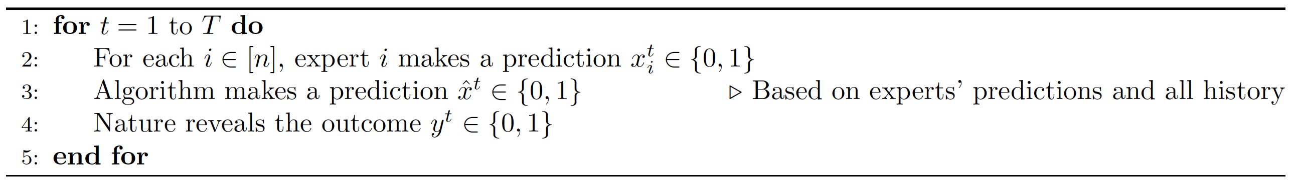
The prediction process involves three parties: the algorithm (player), $n$ experts, and the nature (adversary).
In the esports betting situation we give above, the one who wants to bet is the player, game commentators are experts, and the game itself is the nature.
First, in this section, we consider the most basic situation where experts will only give binary advice (such as “win” or “lose”). The prediction process is formalized into the following algorithm.
For each $i \in [n]$, let $m_i$ be the number of mistakes made by expert $i$, i.e.,
\[m_i = | \{ t \in [T] : x_i^t \neq y^t \} |.\]Let $m^*$ be the number of mistakes made by the best expert; i.e.,
\[m^* = \min_{i \in [n]} m_i.\]Finally, let $\hat{m}$ be the number of mistakes made by the algorithm; i.e.,
\[\hat{m} = | \{ t \in [T] : \hat{x}^t \neq y^t \} |.\]The goal of the algorithm is to minimize $\hat{m}$ compared to $m$. We want to establish that $\hat{m}\leq \alpha m^* + \beta$ where $\alpha, \beta$ may depend on $n,T$.
Ideally, we want to have $ \alpha = 1$ and $ \beta = o_n(T)$, which means that the fraction of mistakes in $T$ rounds made by the algorithm and the best expert are asymptotically the same as T goes to infinity.
Halving Algorithm
As a warm-up, consider the special case where one of the experts is perfect and makes no mistake in all $T$ rounds, and so $m = 0$.
Our goal is to minimize $\hat{m}$. Let $S^t$ be the set of experts that make no mistake up to time $t$. The algorithm maintains the set $S^t$ for all $t$.
In each round of Algorithm 1:
either $\hat{x}^t = y^t$ (the algorithm is correct), in which case we have trivially $\lvert S^t \rvert \leq \lvert S^{t-1} \rvert$;
or $\hat{x}^t \neq y^t$ (the algorithm makes a mistake), in which case we have $\lvert S^t \rvert \leq \frac{1}{2} \lvert S^{t-1} \rvert$ since the majority of the experts in $S^{t-1}$ are wrong and will be excluded from $S^t$.
Therefore, we have
\[\lvert S^t \rvert \leq (\frac{1}{2})^{\hat{m}} \lvert S^{0} \rvert = \frac{n}{2^{\hat{m}}}.\]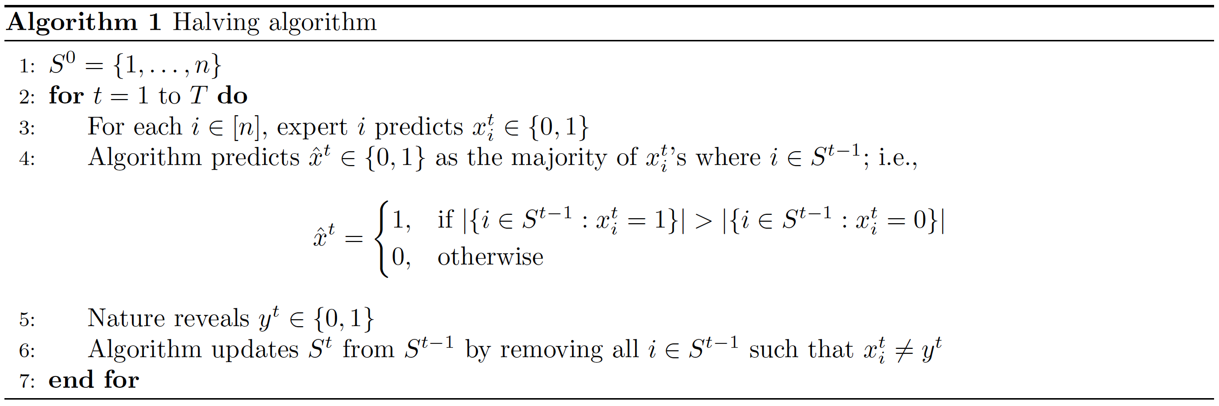
Meanwhile, we have
\[|S^T| \geq 1 ,\]since at least one of the experts is perfect. It follows that
\[1 \leq |S^T| \leq \frac{n}{2^{\hat{m}}} \quad\Longrightarrow \quad \hat{m} \leq \log_2{n}.\]Namely, Algorithm1 makes at most $\log_2{n}$ mistakes, which is independent of $T$.
Weighted Majority Algorithm
In the general case where a perfect expert does not necessarily exist, we maintain a vector $w^t = (w_1^t, …, w_n^t)$ of weights of all experts which represents our confidence/evaluation for each expert. When making a prediction, we use a weighted majority vote among all experts.
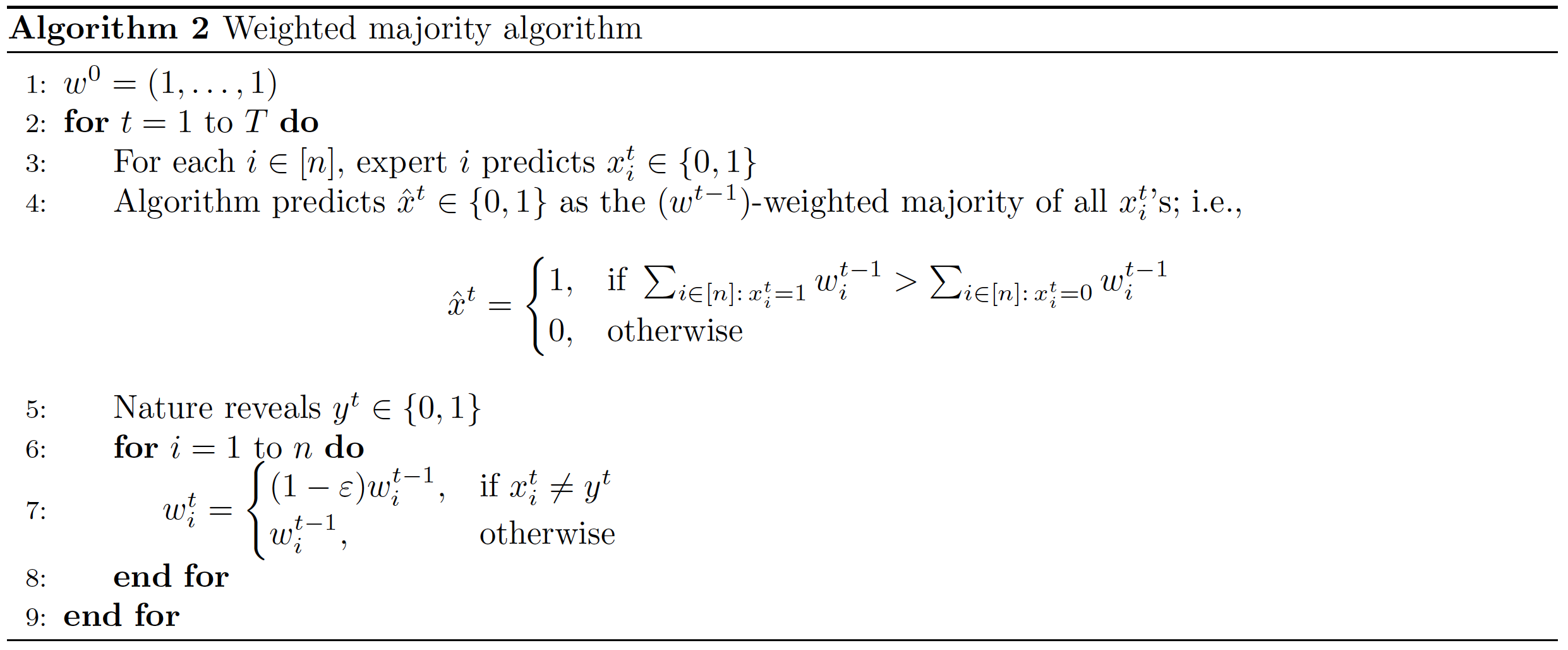
Let $Z^t = \sum_{i=1}^n w_i^t$. In each round of Algorithm 2:
either $\hat{x}^t = y^t$ (the algorithm is correct), in which case we have trivially $ Z^t \leq Z^{t-1} $;
or $\hat{x}^t \neq y^t$ (the algorithm makes a mistake), in which case we have
since the weights of experts who are wrong, which have sum at least $\frac{1}{2}Z^{t-1}$, will decrease by a factor of $1-\varepsilon$.
Therefore, we have
\[Z^T \leq (1 - \frac{1}{2} \varepsilon)^{\hat{m}}Z^{0} = (1 - \frac{1}{2} \varepsilon)^{\hat{m}}n.\]Suppose $i^$ is a best expert with the fewest mistakes (i.e., $i \in \arg \min_{i \in [n]} m_i$), and so $m^ = m_{i^*}$ . Then we have
\[Z^T = \sum_{i=1}^n w_i^T \geq w_{i^*}^T = (1 - \varepsilon)^{m_{i^*}} w_{i^*}^0 = (1 - \varepsilon)^{m^*}.\]It follows that
\[(1 - \varepsilon)^{m^*} \leq Z^T \leq (1-\frac{\varepsilon}{2})^{\hat{m}}n.\]Taking logarithms on both sides, we deduce that
\[m^* \log{\frac{1}{1-\varepsilon}} \geq \hat{m} \log{\frac{1}{1-\varepsilon / 2}} - \log{n}.\]Since we have
\[\log{\frac{1}{1-\varepsilon}} = \varepsilon \pm O(\varepsilon^2) \quad \text{and} \quad \log{\frac{1}{1-\varepsilon / 2}} = \frac{\varepsilon}{2} \pm O(\varepsilon^2),\]we conclude that
\[\hat{m} \leq (2+O(\varepsilon))m^* + O(\frac{\log{n}}{\varepsilon}).\]