There are two normal forms in propositional logic: disjunctive normal form (DNF) and conjunctive normal form (CNF). In the last article, we know that DNF satisfying problem is easy to solve; however, the situation is different as of CNF.
In this article, we will discuss how to gentlely handle the CNF satisfying problem with some acceptible constraint.
2-SAT
A Boolean formula $f$ is in conjunctive normal form (CNF) if it is an AND of ORs, e.g.,
\[f = (x_1 \lor \lnot x_2) \land (\lnot x_2 \lor x_3) \land (x_2 \lor x_4)\]Given a Boolean formula $f$ in CNF where every clause contains exactly two literals (like the example above), we want to find a satisfying assignment for $f$, and this problem is called the 2-SAT problem.
SAT problem for CNF is NP-complete, but 2-SAT can be solved in polynomial time via a reduction to strongly connected components of directed graphs.
Here we present a simple randomized algorithm. Algorithm 1 applies to the general SAT problem and we shall analyze it for 2-SAT.
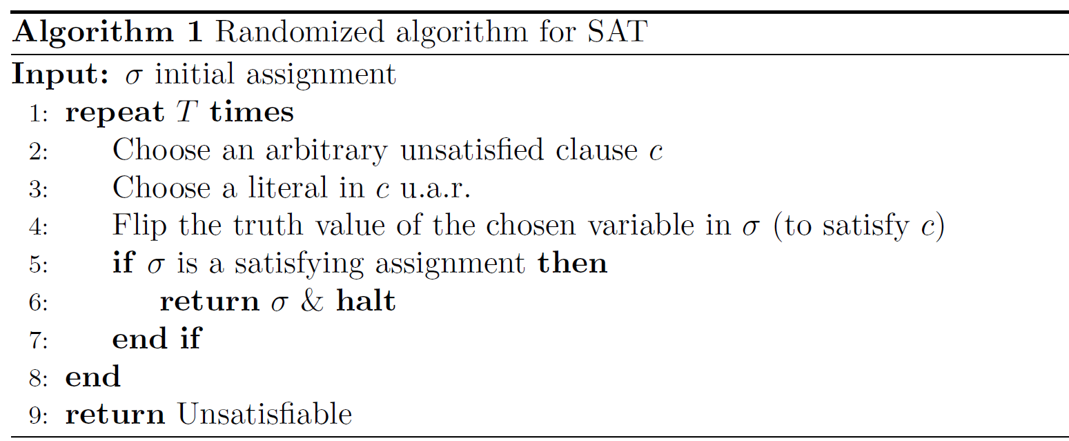
There are some remarks about this algorithm:
We can pick an arbitrary assignment $\sigma$ as initialization, e.g., taking the all-true or all-false assignment. Alternatively, we can apply random initialization: start with a uniformly random assignment $\sigma$.
In Line 2, we can choose the unsatisfied clause $c$ arbitrarily, e.g., picking the one of the smallest index, or choosing one uniformly at random.
In Line 3, we have to choose a literal uniformly at random for our analysis to work.
If f is unsatisfiable, then clearly Algorithm 1 will output Unsatisfiable. Suppose $f$ is satisfiable, and let $\tau$ be a satisfying assignment. Define $\sigma_t$ to be the assignment at time $t$ of Algorithm 1, and $X_t$ to be the number of variables that agree between $\sigma_t$ and $\tau$.
“Agree” means the variable is set to the same truth value in two assignments. For example, suppose $\sigma_t = (\text{T, T, F, T})$ and $\tau = (\text{T, F, F, T})$, we have $X_t = 3$.
If $X_t = n$, then $\sigma_t = \tau$ and the algorithm finds a satisfying assignment.
Note that \(X_t \in \{ 0,1,...,n \}\) can be thought of as a random walk moving between adjacent integers where either $X_{t+1} = X_{t}+1$ or $X_{t+1} = X_{t}-1$ (because each walk will only change the value of one variable!).
Here we have a claim:
For each $t < T$ and \(i \in \{ 0,1,...,n-1 \}\) , we have
\[\Pr(X_{t+1} = i+1 \mid X_t=i) \geq \frac{1}{2}.\](Optional to read) Proof. Suppose we pick clause $c$ in the update from $\sigma_t$ to $\sigma_{t+1}$, and the two variables in $c$ are $x_1$ and $x_2$ without loss of generality. Then, $c$ is not satisfied by $\sigma_t$ but is satisfied by $\tau$. This means that $\sigma_t(x_j) \neq \tau(x_j)$ for at least one \(j \in \{ 1,2 \}\). If $\delta_t(x_1) \neq \tau(x_1)$ and $\delta_t(x_2) = \tau(x_2)$, then $X_{t+1} = X_t + 1$ with probability 1/2. Similarly for the case $\delta_t(x_1) = \tau(x_1)$ and $\delta_t(x_2) \neq \tau(x_2)$. If $\delta_t(x_1) \neq \tau(x_1)$ and $\delta_t(x_2) \neq \tau(x_2)$, then $X_{t+1} = X_t + 1$ always. The claim then follows.
This claim indicates that for each walk we have larger chance to move forward (to the correct answer) than to move backward. Based on this claim, we want to further show that the number of steps for $X_t$ to reach $n$ (in which case $\sigma_t = \tau$) is $\text{poly}(n)$ in expectation.
To simplify the proof, let’s consider a slowed-down process $(Y_t)$ where $Y_0 = X_0$ and
\[\Pr(Y_{t+1} = i+1 \mid Y_t=i) = \frac{1}{2}.\]So, $(Y_t)$ is an unbiased random walk on \(\{ 0,1,...,n \}\). If we can show this slowed-down version can reach $n$ in expected $\text{poly}(n)$ steps, then $(X_t)$ can do as well! And this is what we are going to do.
Define $H_j$ to be the number of steps for the random walk $(Y_t)$ to reach $n$ when starting $Y_0 = j$. Let $h_j = \mathbb{E}[H_j]$ be its expectation. Here comes a key lemma.
(Lemma) For all $j \in { 0,1,…,n }$, we have
\[h_j = n^2 - j^2.\]In particular, $h_j \leq h_0 = n^2$.
Proof. By definition, we have the following recurrence:
\[\begin{cases} h_0 = h_1 + 1;\\ h_j = \frac{1}{2} h_{j-1} + \frac{1}{2} h_{j+1} + 1, \quad 1 \leq j \leq n-1;\\ h_n = 0. \end{cases}\]The first equation holds because one can only move one step forward when in the position 0. The last equation holds because no step is needed when already in the terminal position.
Thus, we have
\[h_j-h_{j+1} = h_{j-1} - h_{j} + 2 = h_{j-2} - h_{j-1} + 4 = \cdots = h_0-h_1+2j = 2j + 1,\]and
\[h_j = h_j-h_n = \sum_{i=j}^{n-1}h_i - h_{i+1} = \sum_{i=j}^{n-1}2i + 1 = n^2-j^2,\]as claimed.
If we run Algorithm 1 with $T = 2n^2$ rounds, then it holds
\[\begin{split} &\Pr(\text{Algorithm 1 outputs Unsatisfiable})\\ \leq &\Pr(X_t \text{ does not reach } n \text{ for } t \leq 2n^2)\\ \leq &\Pr(Y_t \text{ does not reach } n \text{ for } t \leq 2n^2)\\ \leq &\Pr(H_0 > 2n^2)\\ \leq & \frac{h_0}{2n^2} = \frac{1}{2}. \quad \quad \quad \quad \quad \text{(Markov's Inequality)} \end{split}\]The walk we described in this section is so called Markov chain. A Markov chain, simply speaking, is a stochastic process where the outcome of each step is based solely on the present state. More to see this wiki page.
3-SAT
Introduction
In the 3-SAT problem, we are given a Boolean formula $f$ in CNF where every clause contains exactly three literals, and our goal is to find a satisfying assignment for $f$.
Recall that 3-SAT is NP-complete. Moreover, the Exponential Time Hypothesis (ETH) states that 3-SAT cannot be solved in $2^{o(n)}$ time.
The trivial algorithm for 3-SAT is to enumerate all $2^n$ assignments and check for each of them if it is satisfying or not. The running time of such a brute-force algorithm is $2^n\text{ploy}(n)$.
We want to find a faster algorithm running in time $a^n\text{poly}(n)$ for some $a < 2$ as small as possible. In fact, we show that Algorithm 1 with random initialization can achieve $a = 4/3$ for 3-SAT.
Naive Solution
As before, we assume $f$ is satisfiable and let $\tau$ be a satisfying assignment. Define $\sigma_t$ to be the assignment as time $t$ of Algorithm 1, and $X_t$ to be the number of variables that agree between $\sigma_t$ and $\tau$.
Analogously to our previous claim, we have for each $t < T$ and $i \in { 0,1,…,n-1 }$ that
\[\Pr(X_{t+1} = i+1 \mid X_t=i) \geq \frac{1}{3}.\]The slowed-down version $(Y_i)$ is then defined as $Y_0 = X_0$ and
\[\Pr(Y_{t+1} = i+1 \mid Y_t=i) = \frac{1}{3}.\]If $h_j$ denotes the expected number of steps for $(Y_t)$ to reach $n$ starting at $Y_0 = j$, then we have the recurrence
\[\begin{cases} h_0 = h_1 + 1;\\ h_j = \frac{2}{3} h_{j-1} + \frac{1}{3} h_{j+1} + 1, \quad 1 \leq j \leq n-1;\\ h_n = 0. \end{cases}\]Solving the recurrence gives
\[h_j =2^{n+2} - 2^{j+2} - 3(n-j).\]Note that $ h_0 =2^{n+4} - 4 - 3n = \Theta(2^n)$ (for worst case initialization) and $ h_{n/2} =2^{n+2} - 2^{n/2+2} - 3n/2 = \Theta(2^n)$ (for random initialization). Therefore, the previous argument for 2-SAT could only give a $2^n\text{poly}(n)$ time algorithm for 3-SAT!
In fact, even for $j = n-1$ we have $ h_{n-1} =2^{n+2} - 2^{n+1} - 3 = \Theta(2^n)$; namely, even if we start with an assignment $\sigma_0$ which differ from $\tau$ at only one variable, the number of steps to reach $\tau$ could be $\Theta(2^n)$ in expectation.
However, for this special situation, although the expected number of steps is large,the probability of reaching $\tau$ in the first step is at least 1/3; that is, $\Pr(Y_1=n\mid Y_0 = n-1) = 1/3$.
This indicates that, instead of analyzing the expected number of steps to reach $n$ (and then applying the Markov’s inequality), we should look at directly the probability of reaching $n$ within $T$ steps.
Better Solution
We can set $T = 3n$ in Algorithm 1. For any $1 \leq j \leq n$, we deduce that
\[\begin{split} &\Pr(Y_t \text{ reaches } n \text{ for } t \leq 3n \mid Y_0 = n-j)\\ \geq &\Pr(\text{in the first } 3j \text{ steps, } 2j \text{ of them are "+1" and } j \text{ of them are "-1"} \mid Y_0 = n-j) \\ = & C_{j}^{3j} (\frac{1}{3})^{2j} (\frac{2}{3})^{j}\\ \geq & \frac{1}{3j+1} (3)^j (\frac{3}{2})^{2j} (\frac{1}{3})^{2j} (\frac{2}{3})^{j} \quad \quad \quad \quad (\star)\\ \geq &\frac{1}{4n} (3 \cdot \frac{3^2}{2^2} \cdot \frac{1}{3^2} \cdot \frac{2}{3})^j \\ = & \frac{1}{4n} \cdot \frac{1}{2^j} \end{split}\]The inequality used in the $(\star)$ line is based on the following fact:
For any $n \in \mathbb{N}$ and $\alpha \in (0,1)$, such that $\alpha n$ is an integer, we have \(C_{n}^{\alpha n} \geq \frac{1}{n+1} (\frac{1}{\alpha})^{\alpha n}(\frac{1}{1-\alpha})^{(1-\alpha)n}.\)
Recall that in random initialization, we pick the initial assignment $\sigma_0$ unifromly at random. Hence, $X_0 = Y_0$, the number of variables that agree in $\sigma_0$ and $\tau$, is a binomial random variable with parameters $n$ and 1/2. We then deduce that
\[\begin{split} &\Pr(\text{Algorithm 1 finds a satisfying assignment}) \\ \geq & \Pr(X_t \text{ reaches } n \text{ for } t \leq 3n) \\ \geq & \Pr(Y_t \text{ reaches } n \text{ for } t \leq 3n) \\ = &\sum_{j=0}^{n} \Pr(Y_0=n-j) \Pr(Y_t \text{ reaches } n \text{ for } t \leq 3n \mid Y_0 = n - j)\\ \geq &\sum_{j=0}^{n} \frac{C_{n}^{j}}{2^n} \cdot \frac{1}{4n} \cdot \frac{1}{2^j} \\ = &\frac{1}{4n} \cdot \frac{1}{2^n} \sum_{j=0}^{n} C_{n}^{j} \frac{1}{2^j}\\ = &\frac{1}{4n} \cdot \frac{1}{2^n} (1 + \frac{1}{2})^n\\ = & \frac{1}{4n} (\frac{3}{4})^n . \end{split}\]Therefore, repeating Algorithm 1 for $(\frac{4}{3})^n \text{poly}(n)$ times allows us to find a satisfying assignment with probability at least 1/2. The overall running time is $(\frac{4}{3})^n \text{poly}(n)$, which is much better than $2^n$!