Monte Carlo methods, or Monte Carlo experiments, are a broad class of computational algorithms that rely on repeated random sampling to obtain numerical results. This article introduces the application of the Monte Carlo method on the DNF counting problem.
DNF Introduction
A Boolean formula \(f\) is in disjunctive normal form (DNF) if it is an OR of ANDs, e.g.,
\[f = (x_1 \land \lnot x_3 \land x_4) \lor (\lnot x_2 \land x_3) \lor (x_2)\]The Boolean satisfiability problem (also called SAT) is a problem of determining whether there exists an assignment (each either True or False) that results in the formula returning True.
It is easy to find a satisfying assignment for a formula in DNF: Take any clause, and find an assignment that satisfies all literals in that clause. For example, \((x_1, x_2, x_3, x_4) = (\text{T, T, F, T})\) is a satisfying assignment to the formula \(f\) above where the first and third clauses are satisfied.
Here, we use the word “clause” to refer to the terms connected by OR. There are three clauses in our Boolean formula \(f\): \((x_1 \land \lnot x_3 \land x_4)\), \((\lnot x_2 \land x_3)\), and \((x_2)\).
The DNF Counting Problem
Given a Boolean formula \(f\) in DNF with \(n\) variables \(x_1, ..., x_n\) and \(m\) clauses \(c_1, ... ,c_m\), our goal is to find
\[N(f) := \text{number of satisfying assignments of } f\]For example, consider a simple Boolean formula \(f_1 = (x_1 \land \lnot x_2) \lor (x_3)\). We can count \(N(f_1)\) by drawing its truth table.
| \(x_1\) | \(x_2\) | \(x_3\) | \(f_1 = (x_1 \land \lnot x_2) \lor (x_3)\) |
|---|---|---|---|
| T | T | T | T |
| T | T | F | F |
| T | F | T | T |
| T | F | F | T |
| F | T | T | T |
| F | T | F | F |
| F | F | T | T |
| F | F | F | F |
You can see that only five assignments satisfying \(f_1\). So, \(N(f_1)=5\).
Surprisingly, exact counting for \(N(f)\) is #P-complete, which is conjectured to be unsolvable in \(\text{poly}(n,m)\) time. This indicates that counting can be much harder than the corresponding decision problem. We want to have an approximate counting algorithm for this problem.
#P (called “Sharp-P”) is a type of problem that count the number of solutions of a problem in NP. This is obviously NP-hard for problems that are NP-complete, but not necessarily easy for problems in P. #P-complete problems are at least as hard as NP-complete problems. More to read this wiki page.
Given a Boolean formula \(f\) in DNF and an approximation parameter \(\varepsilon \in (0,1)\) as inputs, a randomized algorithm is called a fully polynomial-time randomized approximation scheme (FPRAS) if it outputs \(\hat{N}\) satisfying
\[\Pr((1-\varepsilon)\hat{N} \leq N(f) \leq (1+\varepsilon)\hat{N}) \geq \frac{3}{4}\]in time \(\text{ploy}(n,m,1/\varepsilon)\).
Here are some remarks about FPRAS:
A FPRAS gives the strongest form of approximation. It can achieve \(1 \pm \varepsilon\) approximation for any \(\varepsilon \in (0,1)\), but the running time depends (inverse polynomially) on \(\varepsilon\).
The running time of an FPRAS is fully polynomial in \(n\), \(m\), \(1/\varepsilon\). Note, \(n^3m^{2/\varepsilon}\), \(e^{1/\varepsilon}\), \((nm)^{\log{(1/\varepsilon)}} = (1/\varepsilon)^{\log{(nm)}}\) are not fully polynomial.
We can boost the success probability of an FPRAS to \(1-\delta\) for any (input) failure probability \(\delta \in (0,1)\). This can be achieved by running \(O(\log{(1/\delta)})\) trials of the FPRAS, and taking the median of all outputs (same analysis as the “median of means” approach by Chernoff bounds).
Monte Carlo Method
Let \(\Omega\) be a finite universe with “simple” structure such that we know \(\lvert \Omega \rvert\) and can generate random element from \(\Omega\). Let \(S \subseteq \Omega\) be a subset for which we want to estimate \(\lvert \Omega \rvert\).
To estimate \(\lvert \Omega \rvert\), the Monte Carlo algorithm generates a few independent samples from \(\Omega\) uniformly at random and finds the fraction of samples that lie in \(S\) which approximates \(\lvert S \rvert / \lvert \Omega \rvert\). The detailed algorithm is shown below.
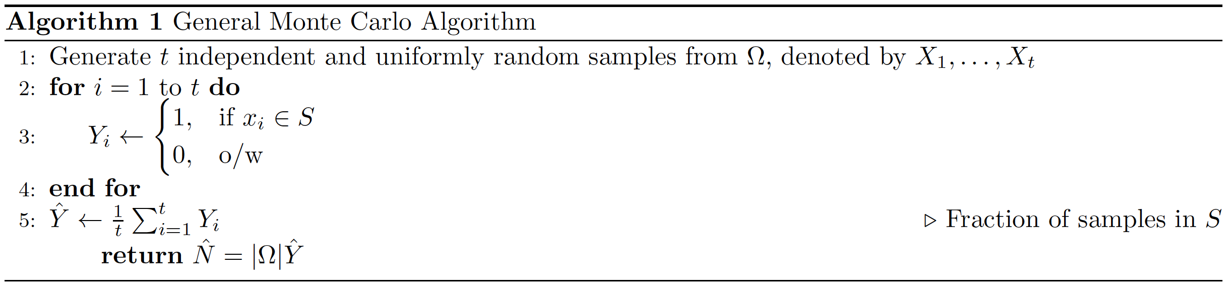
Let \(\alpha = \lvert S \rvert / \lvert \Omega \rvert\), and observe that \(\mathbb{E}[Y_i] = \Pr(X_i \in S) = \lvert S \rvert / \lvert \Omega \rvert = \alpha\) for each \(i\). So, we have \(\mathbb{E}[\hat{Y}] = \alpha\) and \(\mathbb{E}[\hat{N}] = \lvert \Omega \rvert \cdot \mathbb{E}[\hat{Y}] = \alpha \lvert \Omega \rvert = \lvert S \rvert\). This shows that \(\hat{N}\) is an unbiased estimator. By the Chernoff bounds, we deduce that
\[\begin{split} \Pr(|\hat{N}-|S||\geq \varepsilon |S|) &= \Pr(\left|\frac{|\Omega|}{t}\sum_{i=1}^{t}Y_i - |S|\right| \geq \varepsilon |S|) \\ &\leq \Pr(\left|\sum_{i=1}^{t}Y_i - t \alpha \right| \geq \varepsilon (t \alpha) )\\ &\leq 2e^{-\varepsilon^2(t \alpha)/3} \quad \quad \quad \quad \text{(Chernoff Bounds)}\\ &\leq \frac{1}{4} \end{split}\]where the last inequality holds if we set \(t = \lceil \frac{9}{\alpha \varepsilon^2} \rceil\). Hence, we have \(t=\text{poly}(n,m)\) when \(\alpha = \Omega(1/\text{poly}(n,m))\).
For the DNF counting problem, we may define \(\Omega\) to be the set of all truth assignments, so that \(\lvert \Omega \rvert = 2^n\) and we can easily sample an assignment from \(\Omega\) uniformly at random; and we define \(S \subseteq \Omega\) to be the set of satisfying assignments, so \(N(f) = \lvert \Omega \rvert\). Then we can use the Monte Carlo method to directly solve the DNF counting problem.
Note that in the DNF counting problem, we have \(\alpha = N(f)/2^n\). Thus, a straightforward application of Algorithm 1 does not give a polynomial-time algorithm when \(N(f) \ll 2^n\), e.g., \(N(f) \approx 2^{0.99n}\).
Better Monte Carlo Method for DNF Counting
For each clause \(c_i\), let \(S_i\) be the set of assignments that satisfy \(c_i\). Let \(S = \bigcup_{i=1}^{m}S_i\) be the set of all satisfying assignments. Note that \(N(f) = \lvert S \rvert\).
We shall pick the universe \(\Omega\) in a smarter way to apply Algorithm 1. Let \(\Omega\) be the multiset union of \(S_i\)’s; specifically,
\[\Omega = \{ (i, \delta) \in [m] \times S : \sigma \in S_i \}.\]The set \(S\) is technically not a subset of the universe \(\Omega\), but we can easily find a bijective mapping from \(S\) to a subset \(S' \subseteq \Omega\) defined as
\[S'= \{ (i, \delta) \in [m] \times S : \sigma \notin S_i \text{ for } j=1,...,i-1 \text{ and } \delta \in S_i \}\]In other words, \(S'\) consists of all pairs \((i,\delta)\) where \(c_i\) is the first clause satisfied by \(\delta\).
Here are some observations:
\(\lvert S' \rvert = \lvert S \rvert = N(f)\);
\(S' \subseteq \Omega \subseteq [m] \times S\) and so \(\lvert S' \rvert \leq \lvert \Omega \rvert \leq m \lvert S' \rvert\);
For each \(i\), we can easily sample u.a.r. from \(S_i\) by satisfying all the literals in \(c_i\) and choosing a uniformly random assignment for the renaming variables;
For each \(i\), if \(\lvert c_i \rvert = k_i\) (i.e., the clause \(c_i\) contains \(k_i\) literals), then \(\lvert S_i \rvert = 2^{n-k_i}\).
From these observations, we can compute
\[|\Omega| = \sum_{i=1}^{m} |S_i| = \sum_{i=1}^{m} 2^{n-k_i},\]and we can sample uniformly random elements from \(\Omega\) by first sampling \(i \in [m]\) with probability proportional to \(\lvert S_i \rvert\), and then sampling \(\sigma\) u.a.r. from \(S_i\). Algorithm 1 is then specified to the following version.
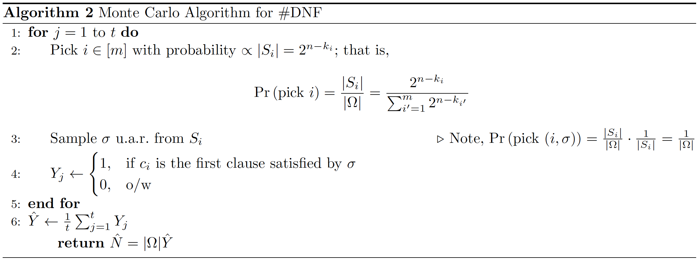
Notice that
\[\mathbb{E}[\hat{Y}] = \alpha = \frac{|S'|}{|\Omega|} \geq \frac{1}{m}\]by our second observation. Therefore, if we set \(t= \lceil \frac{9}{\alpha \varepsilon^2} \rceil = O(\frac{m}{\varepsilon^2})\), then it holds
\[\Pr(\left| \hat{N}-N(f) \right| \geq \varepsilon N(f) ) \leq \frac{1}{4}.\]