Formalization in Software Engineering (1): Reading Sets, Mappings, and Program States

A new master’s student arrives at a paper discussion with question marks all over the methods section. The words variable, state, and assignment are familiar enough. Why has the author introduced a whole new set of symbols to describe them? Each symbol looks manageable on its own, but the formula as a whole is hard to read.

The supervisor points to a definition and asks three questions: What objects are being defined? How are they related? What does this rule do to the program state? Read in that order, the formula begins to look like a compact piece of pseudocode.

This series starts with those three questions. It is written mainly for master’s students new to program analysis, though anyone interested in static analysis, program verification, or programming languages is welcome. You do not need to work through a full mathematics textbook before starting. The aim is to help you read the formal parts of research papers: identify the objects, interpret the rules, and understand the assumptions behind the claims.

The six main articles follow how an analyzer represents and reasons about a program. We start with program states, move on to control flow and semantics, and then use abstract interpretation to cope with large state spaces. Later articles cover fixed-point computation, soundness, and engineering trade-offs. This first article concentrates on reading the notation one piece at a time.

Program objects, relationships, and rules give us a way to connect the notation to the program it describes.

We will identify the basic objects in a formula, see how they form a program state, and translate an assignment rule into words and pseudocode. Here are two expressions we will learn to read:

\[\sigma\in\Sigma=X\rightarrow V\]

and

\[[\![x=e]\!](\sigma) = \sigma[x\mapsto[\![e]\!](\sigma)].\]

There is no unknown to solve for here. The first expression defines a program state; the second describes how assignment changes that state. Once we unpack them, the operations are much like dictionary lookups and updates. These are the kinds of definitions you will encounter in papers at ICSE, FSE, ASE, and ISSTA.

In many software engineering papers, formalization provides a precise language for answering three questions:

1. What objects are we studying?
2. How are those objects organized?
3. What rules does the method use to process them?

We will work toward a small program with just two assignments. Along the way, we will distinguish sets, elements, tuples, and sequences, use mappings to represent program states, and read a semantic rule as a few steps of pseudocode. You do not need to memorize a table of symbols. You need a reading order that still works when the symbols are unfamiliar.

---

1. What is formalization for?

Consider this description of an analyzer:

The analyzer records the value of each variable as the program executes.

The sentence is easy to follow, but it leaves several questions open:

• Which objects count as variables?
• What values can they take?
• Does every variable have a value?
• How is an unknown value represented?
• What mathematical relationship does “records” describe?

The author might begin by defining

\[X = \text{the set of program variables},\] \[V = \text{the set of values},\]

and then write

\[\sigma:X\rightarrow V.\]

This says that $\sigma$ is a mapping from the set of variables $X$ to the set of values $V$. For any variable $x\in X$, $\sigma(x)$ is its value in that state.

The prose explains the idea; the formal definition makes the relationship precise. A well-written paper usually gives you both.

When you first see

\[\sigma\in\Sigma=X\rightarrow V,\]

you may be tempted to look for a derivation. But this line combines several definitions. Read it from right to left:

1. $X\rightarrow V$: functions from $X$ to $V$.
2. $\Sigma=X\rightarrow V$: $\Sigma$ is the set of all such functions.
3. $\sigma\in\Sigma$: $\sigma$ is one particular function in that set.

Together, they say:

A program state $\sigma$ maps each variable to a value.

When you meet a formula, first try to say it in ordinary language. Then ask why the author chose that definition.

---

2. The basic objects in a formula

Many complicated definitions are built from a few familiar structures. Sets collect objects, tuples combine them into records, and sequences keep them in order.

2.1 Sets and elements

Suppose

\[X=\text{the set of program variables}.\]

$X$ might contain

\[X=\{x,y,result,count,\ldots\}.\]

A paper will rarely list every variable in the program. It uses $X$ to refer to the set as a whole.

Membership: $x\in X$.

The expression

\[x\in X\]

says that $x$ is an element of $X$. If $X$ has already been defined as the set of variables, you can simply read it as “$x$ is a variable.”

Similarly, if

\[L=\text{the set of program locations},\]

then

\[\ell\in L\]

says that $\ell$ is a program location.

Uppercase and lowercase letters are a convention.

Program analysis and programming language papers often write

\[x\in X,\qquad v\in V,\qquad \ell\in L.\]

An uppercase letter commonly names a set or domain; a lowercase letter names one of its elements. For example, $V=\mathbb{Z}$ says that the value domain is the integers, while $v\in V$ denotes a particular integer.

This is a naming convention, not a mathematical rule. Always check the author’s definition.

2.2 Tuples, Cartesian products, and sequences

In the expression

\[A\times B,\]

$\times$ usually denotes the Cartesian product. It forms pairs by taking one element from $A$ and one from $B$.

If

\[A=\{a_1,a_2\},\qquad B=\{b_1,b_2\},\]

then

\[A\times B= \{(a_1,b_1),(a_1,b_2),(a_2,b_1),(a_2,b_2)\}.\]

In program analysis, a Cartesian product often combines different kinds of information. For example,

\[L\times X\]

is the set of all pairs of program locations and variables. A pair $(\ell,x)$ identifies variable $x$ at location $\ell$. Add the value domain, and

\[(\ell,x,v)\in L\times X\times V\]

can record that, at program location $\ell$, variable $x$ has value $v$.

When you see $\times$, think of combining objects into a tuple.

A tuple has a fixed number of components, each with its own role. When the number of elements can vary and their order matters, a sequence is often more appropriate.

The notation

\[A^*\]

denotes the set of finite sequences containing zero or more elements from $A$. The star is called the Kleene star.

If $I$ is the set of instructions, then members of $I^*$ include

\[[],\qquad [i_1],\qquad [i_1,i_2,i_3].\]

You may see this notation used for

• sequences of statements or instructions;
• function argument lists;
• application programming interface (API) call sequences;
• execution traces.

A set tells you which objects belong to a collection. A tuple combines objects into one record. A sequence records their order and may have any finite length, including zero.

---

3. Representing program states with mappings

Once we know the basic objects, we can describe the relationships between them. Mappings are one of the most common ways to do this.

3.1 From a function declaration to a program state

The expression

\[f:A\rightarrow B\]

says that $f$ is a function from $A$ to $B$. Given $a\in A$, the result $f(a)$ belongs to $B$.

For example, let

\[Name=\{Alice,Bob,Carol\},\qquad Age=\mathbb{N}.\]

We can define

\[age:Name\rightarrow Age.\]

For example, $age(Alice)=20$ says that Alice is 20 years old.

When reading a function declaration, leave its implementation aside at first. Look at the two sides of the arrow: what goes in, and what comes out?

One important use of mappings in program analysis is to associate variables with their current values. A typical definition of a program state is

\[\sigma\in\Sigma=X\rightarrow V.\]

Here,

• $X$ is the set of variables;
• $V$ is the set of values;
• $\Sigma$ is the set of all program states;
• $\sigma$ is one particular program state.

For example,

\[\sigma=\{x\mapsto1,\ y\mapsto3,\ z\mapsto10\}.\]

Then

\[\sigma(x)=1,\qquad \sigma(y)=3,\qquad \sigma(z)=10.\]

In code, this looks much like a dictionary:

state = {
    "x": 1,
    "y": 3,
    "z": 10,
}

For now, you can think of $\sigma:X\rightarrow V$ as

Map<Variable, Value>

Many analyzers maintain data structures much like this one. The formal state definition tells you what those structures represent.

This is a deliberately simple model: every variable has a value, and the state records only those values. Modeling uninitialized variables, objects, or heap memory requires additional structure.

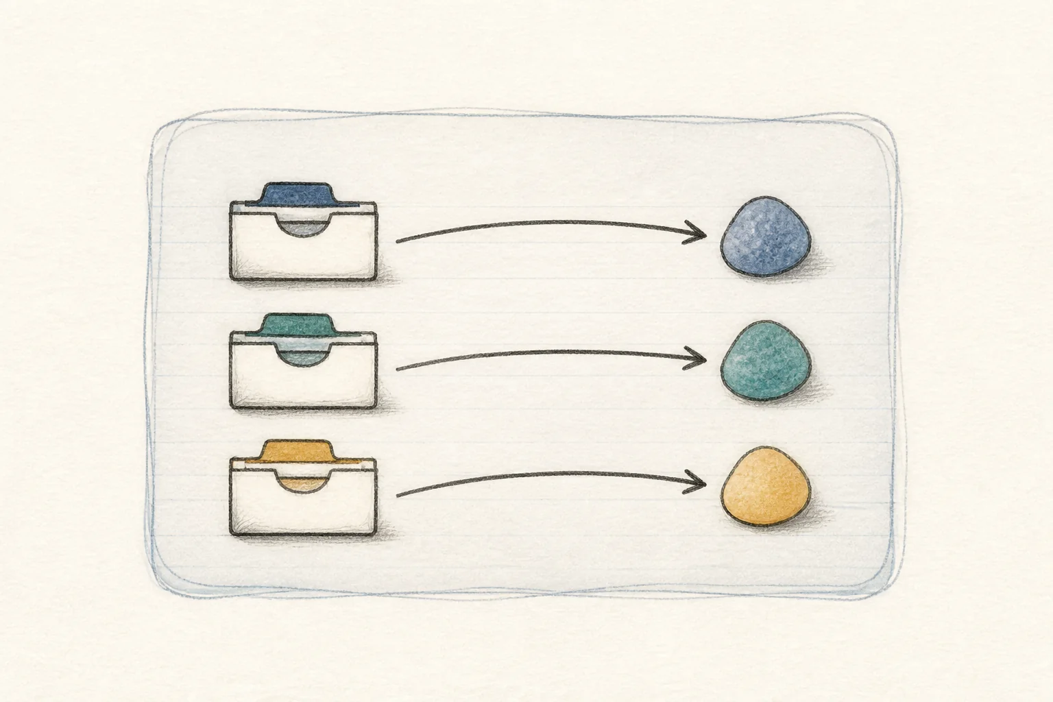
Think of each variable as an index card pointing to its current value. Together, the cards form a snapshot of the program state.

3.2 Arrows, individual mappings, and state updates

These two arrows have different jobs.

$\rightarrow$ describes the type of a mapping.

\[\sigma:X\rightarrow V\]

The inputs to $\sigma$ come from $X$, and its outputs belong to $V$.

$\mapsto$ describes an individual association.

\[x\mapsto42\]

This maps $x$ to 42. Thus,

\[\sigma=\{x\mapsto1,\ y\mapsto2\}\]

gives the contents of a particular state.

$\rightarrow$ tells you the function’s input and output domains; $\mapsto$ tells you what a particular element maps to.

With that distinction in place, we can describe what happens when execution changes a variable’s value.

The expression

\[\sigma[x\mapsto v]\]

denotes a state obtained from $\sigma$ by updating $x$ to $v$ and leaving every other variable unchanged.

If

\[\sigma=\{x\mapsto1,\ y\mapsto2\},\]

then

\[\sigma[x\mapsto10]=\{x\mapsto10,\ y\mapsto2\}.\]

The corresponding pseudocode is

new_state = state.copy()
new_state[x] = 10

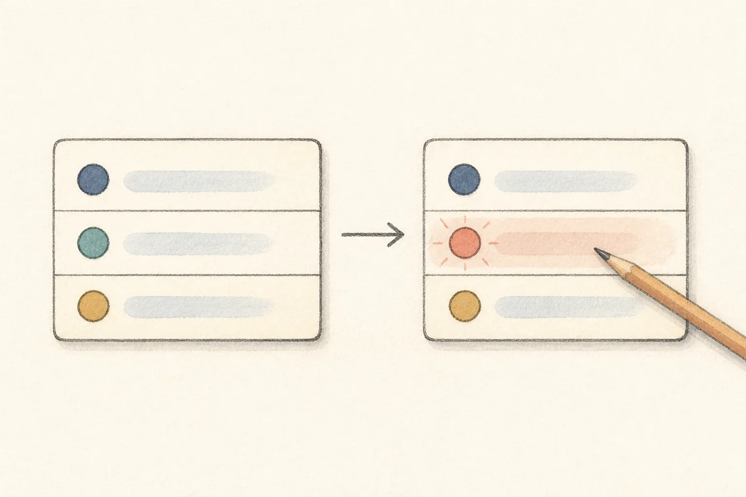
An update replaces one association. The target variable gets a new value; the other variables keep theirs.

Consider the assignment

x = y + 1;

Starting from state $\sigma$, execution proceeds as follows:

1. Read y using $\sigma(y)$.
2. Compute $\sigma(y)+1$.
3. Produce the new state $\sigma[x\mapsto\sigma(y)+1]$.

The notation follows the same steps as the code: evaluate the right-hand side, then store the result in x.

3.3 Naming the updated state

$\sigma’$ is read as “sigma prime.” In program semantics, it often denotes the next or updated state. For example,

\[\sigma\rightarrow\sigma'\]

may describe a transition from state $\sigma$ to state $\sigma’$.

The prime does not have one meaning across all papers. It can also mean another object related to the original one, so check the definition in context.

---

4. From execution to semantic rules

Sets and mappings let us describe states. Semantic rules explain how a piece of code reads or changes them.

4.1 Semantic brackets and the assignment rule

In programming language literature,

\[[\![e]\!]\]

often denotes the semantics of a program construct $e$: what $e$ means. For example,

\[[\![1+2]\!]=3.\]

The result of an expression usually depends on the current state. For x + 1, we can define

\[[\![x+1]\!](\sigma)=\sigma(x)+1.\]

To interpret x + 1 in state $\sigma$, read the value of x and add 1.

When you first meet these brackets, it helps to think of

\[[\![e]\!](\sigma)\]

as

eval(e, state)

Here eval is pseudocode for an expression evaluator, rather than a call to Python’s built-in eval. It takes an expression and a program state and returns the expression’s value.

We can now combine the notation into a complete assignment rule:

\[[\![x=e]\!](\sigma) = \sigma[x\mapsto[\![e]\!](\sigma)].\]

This describes the assignment x = e. Read it in two steps.

Step 1: Evaluate the right-hand side.

\[v=[\![e]\!](\sigma).\]

Evaluate $e$ in the current state $\sigma$ and call the result $v$.

Step 2: Update the state with the result.

\[\sigma[x\mapsto v].\]

Update $x$ to $v$, leaving all other variables unchanged.

The whole rule corresponds to these lines of pseudocode:

value = eval(e, state)
new_state = state.copy()
new_state[x] = value
return new_state

Many semantic rules describe the steps of an interpreter or an analysis algorithm in mathematical notation. Writing out the pseudocode can make the evaluation order easier to follow.

4.2 A complete example: two assignments

Consider this program:

x = 1;
y = x + 2;

Its variable set and value domain are

\[X=\{x,y\},\qquad V=\mathbb{Z}.\]

The set of all program states is

\[\Sigma=X\rightarrow V.\]

Let the initial state be $\sigma_0$. After executing x = 1,

\[\sigma_1=\sigma_0[x\mapsto1],\]

so $\sigma_1(x)=1$.

Next, execute y = x + 2. First evaluate the right-hand side:

\[[\![x+2]\!](\sigma_1) =\sigma_1(x)+2 =3.\]

Then update y:

\[\sigma_2=\sigma_1[y\mapsto3].\]

The final state satisfies

\[\sigma_2(x)=1, \qquad \sigma_2(y)=3.\]

The example connects the definitions to execution: a state records the variable values, and the assignment rule tells us how each statement updates them.

Once concrete execution makes sense, it is easier to see what a static analysis might choose to keep from it. This brings us to another common convention: a hat over a symbol, as in $v$ and $\hat{v}$, often distinguishes an abstract object from a concrete one.

Suppose the concrete value at run time is

\[v=42.\]

If an analyzer only tracks whether a value is positive, negative, or zero, it may represent that value as

\[\hat{v}=Positive.\]

Similarly, $V$ may denote the concrete value domain and $\hat{V}$ the abstract value domain. The analysis keeps the property it needs while discarding some detail:

\[\text{concrete object}\longrightarrow\text{abstract object retaining the properties of interest}.\]

A hat is a common convention in abstract interpretation, but its meaning still depends on the paper. When you see $\hat{x}$, check whether the author is distinguishing concrete and abstract objects.

---

5. Reading an unfamiliar formal definition

The longest rule on the page tends to catch your eye. It is rarely the best place to start. Try the following order instead.

Identify the objects first, follow the relationships between them, then read the rules that perform the computation.

5.1 A reading order you can reuse

Step 1: Find the basic domains.

Look in the prose or the notation table for definitions such as

\[X=?,\qquad V=?,\qquad L=?\]

What basic objects has the author introduced? They may include variables, values, program locations, expressions, and instructions.

Step 2: Find the structured objects.

Look at how the basic objects are combined. For example,

\[\sigma:X\rightarrow V\]

organizes variables and values into a state, while

\[(\ell,\sigma)\in L\times\Sigma\]

combines a program location and a current state into a configuration.

Step 3: Read the function’s inputs and outputs.

Suppose a paper defines

\[Analysis:P\rightarrow R.\]

On the first pass, leave the internals alone. Find out what program representation $P$ denotes and what kind of analysis result $R$ contains. The function’s type already tells you something about the method’s purpose.

Step 4: Read the rules.

Break each rule into its evaluation steps. What does it read? What does it compute? What does it update or return? Write the steps as pseudocode if that helps.

5.2 Keep a notation table, and check the conventions

For a paper with many symbols, a few notes can save a lot of backtracking:

L  = set of program locations
ℓ  = a program location

X  = set of variables
x  = a variable

V  = set of values
v  = a value

Σ  = set of program states
σ  = a program state: a mapping from variables to values

Now you can read $(\ell,\sigma)$ as “the current program location and state” without looking up both symbols again.

Avoid guessing a symbol’s meaning from its appearance. Papers often use

\[\sigma,\pi,\xi,\Gamma,\Sigma,\Phi,\Delta,\ldots\]

Some conventions are widespread: $\sigma$ for a state, $\pi$ for a path, and $\Gamma$ for an environment or context. None of these has a single meaning throughout the field.

If a paper writes $\sigma\in\Sigma$, what matters is how that paper defines $\Sigma$.

5.3 Three common mistakes

Starting with the longest formula.

If you jump straight into the right-hand side of $F(\sigma,\ell,x,\ldots)=\ldots$, undefined symbols can stop you almost immediately. Find the basic domains, function types, and helper definitions first.

Trying to understand every branch on the first pass.

Begin with the main flow:

\[\text{input}\rightarrow\text{state}\rightarrow\text{rule}\rightarrow\text{output}.\]

Once you understand that, return to the boundary cases and special branches.

Treating every formal definition as a proof.

Many formulas in program analysis papers specify how a method works. First ask what the definition describes. Then ask what the author can prove about it.

---

6. A notation reference

Symbol	How to read it
$x\in X$	$x$ is an element of $X$
$A\subseteq B$	$A$ is a subset of $B$
$A\times B$	Pairs with one element from $A$ and one from $B$
$f:A\rightarrow B$	$f$ is a mapping from $A$ to $B$
$x\mapsto v$	$x$ maps to the particular value $v$
$A^*$	The set of finite sequences of elements from $A$
$\sigma:X\rightarrow V$	A program state maps variables to values
$\sigma(x)$	Look up the value of $x$ in the state
$\sigma[x\mapsto v]$	Update $x$ to $v$ in the state
$\sigma’$	Often an updated or next state
$\hat{x}$	Often an abstract version of $x$
\([\![e]\!]\)	The semantic interpretation of program construct $e$

Use this as a reference rather than a list to memorize. You will learn more by interpreting the symbols in the context of a paper.

---

7. Further reading

This article focuses on reading notation. For a closer look at the underlying ideas, choose a resource that fits your research question.

• Programming language foundations: The Easy Foundations for Programming Languages series on this blog begins with the typed $\lambda$-calculus and is intended for students new to programming language theory.

• Formal reasoning and program verification: Software Foundations is an interactive textbook series covering logic, operational semantics, Hoare logic, and type systems. Its definitions and exercises are checked with a proof assistant (Coq), making it a useful place to practice formal reasoning.

• Operational and denotational semantics: The Cornell CS 4110 lecture slides offer a useful distinction: operational semantics describes how a program computes, while denotational semantics describes what it computes. Turn here when a paper introduces evaluation relations or semantic functions.

• An introductory course on static analysis (in Chinese): Yue Li’s Software Analysis course at Nanjing University moves from basic concepts to the theory and practice of static analysis. If you are comfortable studying in Chinese, it offers an accessible introduction for graduate students and interested undergraduates.

• A textbook on static analysis: Once you have some intuition, Introduction to Static Analysis: An Abstract Interpretation Perspective connects program semantics, state abstraction, and abstract semantics to fixed-point computation and worklist algorithms.

• The foundations of abstract interpretation: Patrick Cousot’s MIT course on abstract interpretation goes further into lattices, fixed points, and sound approximation. It is easier to approach once you are comfortable with programs, states, and transition rules.

These resources serve different purposes. For program verification, start with Software Foundations. For static analysis, the MIT Press textbook develops the ideas introduced here; the Nanjing course provides another introduction if you read Chinese. If your immediate goal is to follow semantic definitions in papers, this series and the Cornell materials are reasonable next steps.

---

8. What to take away

A useful first habit is to read in this order:

\[\boxed{ \text{objects} \longrightarrow \text{relationships} \longrightarrow \text{rules} }\]

In a paper, that means asking:

1. What objects has the author defined?
2. How do sets, tuples, and mappings organize those objects?
3. How does the algorithm query, transform, or update those structures?

For the kinds of definitions we have read here, a useful starting intuition is

\[\text{formalization} \approx \text{describing an algorithm precisely with sets, mappings, and rules}.\]

When you see

\[\sigma:X\rightarrow V,\]

read it as

A program state maps each variable to a value.

When you see

\[[\![x=e]\!](\sigma) = \sigma[x\mapsto[\![e]\!](\sigma)],\]

read it as

Evaluate the right-hand side, then update $x$ with the result.

Being able to move between the formula, its meaning in words, and a few lines of pseudocode is a good first step toward reading the formal definitions in software engineering papers.

Back to the series guide · Next: Where Can a Program Go? From Code and CFGs to Program Semantics.